13.2 The Correlation Coefficient
The numerical measure that assesses the strength of a linear relationship is called the correlation coefficient, and is denoted by \(r\). We will:
- give a definition of the correlation \(r\),
- discuss the calculation of \(r\),
- explain how to interpret the value of \(r\), and
- talk about some of the properties of \(r\).
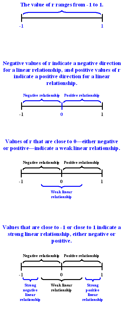
Definition: The correlation coefficient (\(r\)) is a numerical measure that measures the strength and direction of a linear relationship between two quantitative variables.
Calculation: \(r\) is calculated using the following formula: \(r = \frac{1}{n-1}\sum_{i=1}^n \left(\frac{x_i - \bar{x}}{s_x}\right)\left(\frac{y_i - \bar{y}}{s_y}\right)\)
However, the calculation of the correlation (\(r\)) is not the focus of this course. We will use a statistics package to calculate \(r\) for us, and the emphasis of this course will be on the interpretation of its value.
Interpretation
Once we obtain the value of \(r\), its interpretation with respect to the strength of linear relationships is quite simple, as this walk-through will illustrate:
In order to get a better sense for how the value of r relates to the strength of the linear relationship, take a look at this applet.
The slider bar at the bottom of the applet allows us to vary the value of the correlation coefficient (\(r\)) between -1 and 1 in order to observe the effect on a scatterplot. (If the plot does not change on your browser when you move the slider, click along the bar instead to update the plot).
Now that we understand the use of r as a numerical measure for assessing the direction and strength of linear relationships between quantitative variables, we will look at a few examples.
Example
Highway Sign Visibility
Earlier, we used the scatterplot below to find a negative linear relationship between the age of a driver and the maximum distance at which a highway sign was legible. What about the strength of the relationship? It turns out that the correlation between the two variables is \(r = -0.8012447\).
cor(signdist$Age, signdist$Distance)[1] -0.8012447cor.test(signdist$Age, signdist$Distance)
    Pearson's product-moment correlation

data:  signdist$Age and signdist$Distance
t = -7.086, df = 28, p-value = 1.041e-07
alternative hypothesis: true correlation is not equal to 0
95 percent confidence interval:
 -0.9013320 -0.6199255
sample estimates:
       cor
-0.8012447 ggplot(data = signdist, aes(x = Age, y = Distance)) +
geom_point(color = "purple") +
theme_bw() +
labs(x = "Drivers Age (years)", y = "Sign Legibility Distance (feet)") +
stat_smooth(method = lm)
Since \(r < 0\), it confirms that the direction of the relationship is negative (although we really didn’t need \(r\) to tell us that). Since \(r\) is relatively close to -1, it suggests that the relationship is moderately strong. In context, the negative correlation confirms that the maximum distance at which a sign is legible generally decreases with age. Since the value of \(r\) indicates that the linear relationship is moderately strong, but not perfect, we can expect the maximum distance to vary somewhat, even among drivers of the same age.
Example
Statistics Courses
A statistics department is interested in tracking the progress of its students from entry until graduation. As part of the study, the department tabulates the performance of 10 students in an introductory course and in an upper-level course required for graduation. What is the relationship between the students’ course averages in the two courses? Here is the scatterplot for the data:
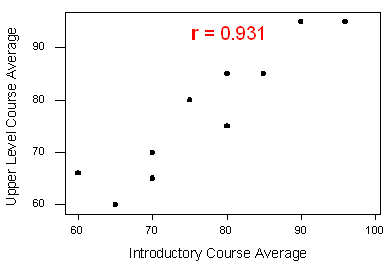
The scatterplot suggests a relationship that is positive in direction, linear in form, and seems quite strong. The value of the correlation that we find between the two variables is \(r = 0.931\), which is very close to 1, and thus confirms that indeed the linear relationship is very strong.
Pearson Correlation
A correlation coefficient assesses the degree of linear relationship between two variables. It ranges from \(+1\) to \(-1\). A correlation of \(+1\) means that there is a perfect, positive, linear relationship between the two variables. A correlation of \(-1\) means there is a perfect, negative linear relationship between the two variables. In both cases, knowing the value of one variable, you can perfectly predict the value of the second.
Pearson Correlation Assignment
Post syntax to your private GitHub repo used to generate a correlation coefficient along with corresponding output and a few sentences of interpretation.
Note: When we square \(r\), it tells us what proportion of the variability in one variable is described by variation in the second variable (aka \(R^2\) or Coefficient of Determination).
Example of how to write results for correlation coefficient: Among daily, young adult smokers (my sample), the correlation between number of cigarettes smoked per day (quantitative) and number of nicotine dependence symptoms experienced in the past year (quantitative) was 0.2593625 (p < 0.0001), suggesting that only 6.73% (i.e. 0.2593625 squared) of the variance in number of current nicotine dependence symptoms can be explained by number of cigarettes smoked per day.
ggplot(data = nesarc, aes(x = DailyCigsSmoked, y = NumberNicotineSymptoms)) +
  geom_point(color = "lightblue") +
  theme_bw() +
  labs(x = "Number of cigarettes smoked daily", y = "Number of nicotine dependence symptoms")
cor.test(nesarc$DailyCigsSmoked, nesarc$NumberNicotineSymptoms)
    Pearson's product-moment correlation

data:  nesarc$DailyCigsSmoked and nesarc$NumberNicotineSymptoms
t = 9.7311, df = 1313, p-value < 2.2e-16
alternative hypothesis: true correlation is not equal to 0
95 percent confidence interval:
 0.2082242 0.3090866
sample estimates:
      cor
0.2593625
r <- cor(nesarc$DailyCigsSmoked, nesarc$NumberNicotineSymptoms, use = "complete.obs")
r[1] 0.2593625r^2[1] 0.0672689