11.5 Post Hoc Tests
When testing the relationship between your explanatory (\(X\)) and response variable (\(Y\)) in the context of ANOVA, your categorical explanatory variable (\(X\)) may have more than two levels.
For example, when we examine the differences in mean GPA (\(Y\)) across different college years (\(X\) = freshman, sophomore, junior and senior) or the differences in mean frustration level (\(Y\)) by college major (\(X\) = Business, English, Mathematics, Psychology), there is just one alternative hypothesis, which claims that there is a relationship between \(X\) and \(Y\).
When the null hypothesis is rejected, the conclusion is that not all the means are equal.
Note that there are many ways for \(\mu_1, \mu_2, \mu_3, \mu_4\) not to be all equal, and \(\mu_1 \neq \mu_2 \neq \mu_3 \neq \mu_4\) is just one of them. Another way could be \(\mu_1 = \mu_2 = \mu_3 \neq \mu_4\) or \(\mu_1 = \mu_2 \neq \mu_3 \neq \mu_4\)
In the case where the explanatory variable (\(X\)) represents more than two groups, a significant ANOVA F test does not tell us which groups are different from the others.
To determine which groups are different from the others, we would need to perform post hoc tests. These tests, done after the ANOVA, are generally termed post hoc paired comparisons.
Post hoc paired comparisons (meaning “after the fact” or “afterdata collection”) must be conducted in a particular way in order to prevent excessive Type I error.
Type I error occurs when you make an incorrect decision about the null hypothesis. Specifically, this type of error is made when your p-value makes you reject the null hypothesis (\(H_0\)) when it is true. In other words, your p-value is sufficiently small for you to say that there is a real association, despite the fact that the differences you see are due to chance alone. The type I error rate equals your p-value and is denoted by the Greek letter \(\alpha\) (alpha).
Although a Type I Error rate of 0.05 is considered acceptable (i.e. it is acceptable that 5 times out of 100 you will reject the null hypothesis when it is true), higher Type I error rates are not considered acceptable. If you were to use the significance level of 0.05 across multiple paired comparisons (for example, three independent comparisons) with \(\alpha = 0 .05\), then the \(\alpha\) rate across all three comparisons is \(1 - (1 - \alpha)^{\text{Number of comparisons}} = 1 - (1 - 0.05)^3 = 0.142625\). In other words, across the unprotected paired comparisons you will reject the null hypothesis when it is true roughly 14 times out of 100.
The purpose of running protected post hoc tests is that they allow you to conduct multiple paired comparisons without inflating the Type I Error rate.
For ANOVA, you can use one of several post hoc tests, each which control for Type I Error, while performing paired comparisons (Duncan Multiple Range test, Dunnett’s Multiple Comparison test, Newman-Keuls test, Scheffe’s test, Tukey’s HSD test, Fisher’s LSD test, Sidak).
Analysis of Variance
Analysis of variance assesses whether the means of two or more groups are statistically different from each other. This analysis is appropriate when you want to compare the means (quantitative variables) of \(k\) groups (categorical variables) under certain assumptions (constant variance for all \(k\) groups). The null hypothesis is that there is no difference in the mean of the quantitative variable across groups (categorical variable), while the alternative is that there is a difference.
TukeyHSD(aov(Frustration.Score ~ Major, data = frustration)) Tukey multiple comparisons of means
95% family-wise confidence level
Fit: aov(formula = Frustration.Score ~ Major, data = frustration)
$Major
diff lwr upr p adj
English-Business 4.4571429 2.8449899 6.069296 0.0000000
Mathematics-Business 5.8857143 4.2735614 7.497867 0.0000000
Psychology-Business 6.7142857 5.1021328 8.326439 0.0000000
Mathematics-English 1.4285714 -0.1835815 3.040724 0.1019527
Psychology-English 2.2571429 0.6449899 3.869296 0.0021515
Psychology-Mathematics 0.8285714 -0.7835815 2.440724 0.5411978opar <- par(no.readonly = TRUE)
par(mar = c(5.1, 11.1, 4.1, 2.1), las = 1) # Enlarge left margin
plot(TukeyHSD(aov(Frustration.Score ~ Major, data = frustration)))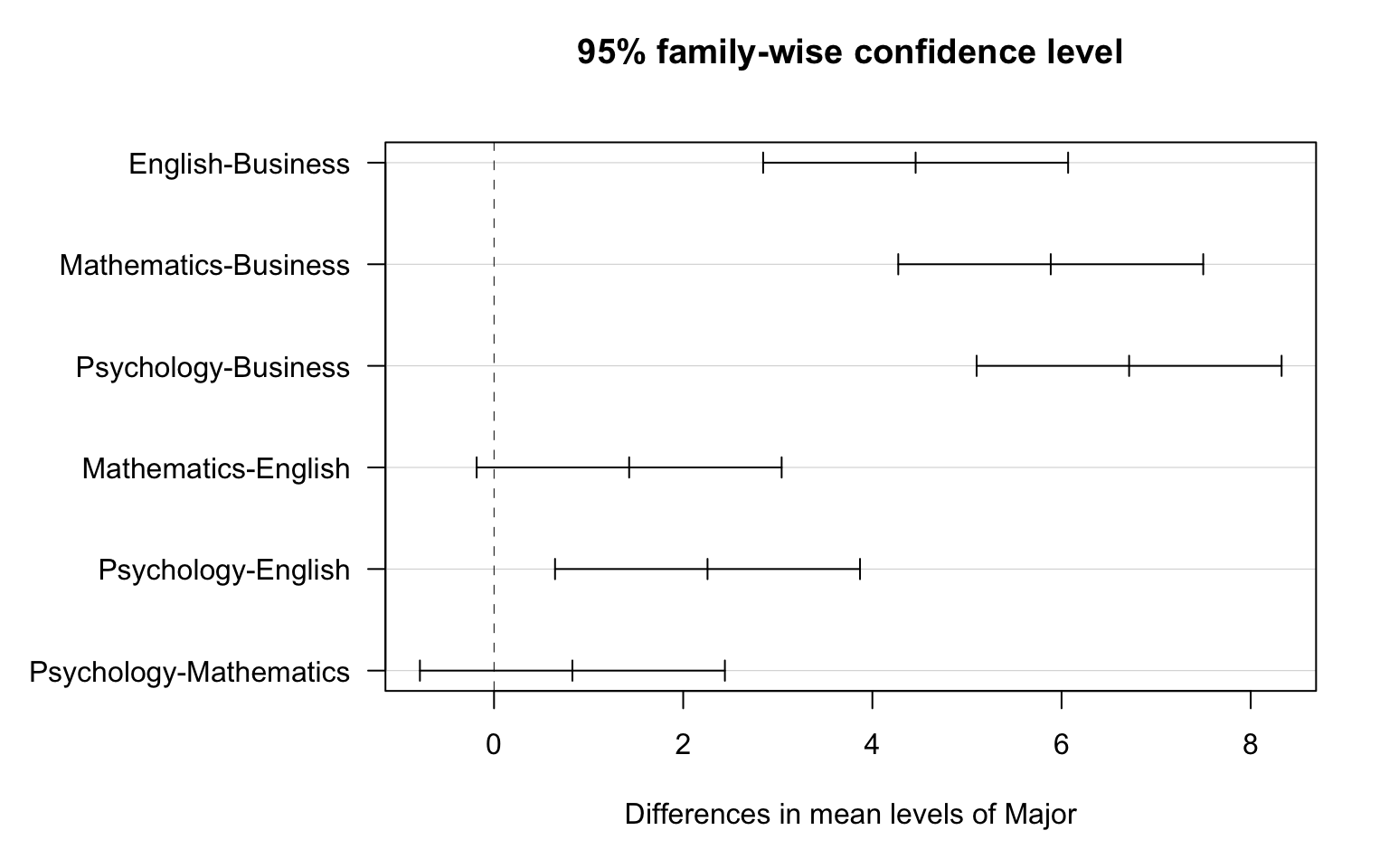
par(opar) # reset marginsOf the \(\binom{4}{2}=6\) pairwise differences, Tukey’s HSD suggest that all except Mathematics - English and Psychology - Mathematics are significant.
Analysis of Variance Assignment
Post the syntax to your private GitHub repository used to run an ANOVA along with corresponding output and a few sentences of interpretation. You will need to analyze and interpret post hoc paired comparisons in instances where your original statistical test was significant, and you were examining more than two groups (i.e. more than two levels of a categorical, explanatory variable).
Example of how to write results for ANOVA:
MEANS <- tapply(nesarc$DailyCigsSmoked, list(nesarc$TobaccoDependence), mean, na.rm = TRUE)
MEANS
No Nicotine Dependence Nicotine Dependence
11.41393 14.62782 SD <- tapply(nesarc$DailyCigsSmoked, list(nesarc$TobaccoDependence), sd, na.rm = TRUE)
SDNo Nicotine Dependence Nicotine Dependence
7.427612 9.152854 RES <- summary(aov(DailyCigsSmoked ~ TobaccoDependence, data = nesarc))
RES Df Sum Sq Mean Sq F value Pr(>F)
TobaccoDependence 1 3241 3241 44.68 3.42e-11 ***
Residuals 1313 95236 73
---
Signif. codes: 0 '***' 0.001 '**' 0.01 '*' 0.05 '.' 0.1 ' ' 1
5 observations deleted due to missingnessWhen examining the association between current number of cigarettes smoked (quantitative response) and past year nicotine dependence (categorical explanatory), an Analysis of Variance (ANOVA) revealed that among daily, young adult smokers (my sample), those with nicotine dependence reported smoking significantly more cigarettes per day (Mean = 14.6, s.d. \(\pm\) 9.2) compared to those without nicotine dependence (Mean = 11.4, s.d. \(\pm\) 7.4), F(1, 1313) = 44.7, p < 0.0001.
Example of how to write post hoc ANOVA results:
nesarc$DCScat <- cut(nesarc$DailyCigsSmoked, breaks = c(0, 5, 10, 15, 20, 98), include.lowest = FALSE)
mod <- aov(NumberNicotineSymptoms ~ DCScat, data = nesarc)
RES <- summary(mod)
RES
Df Sum Sq Mean Sq F value Pr(>F)
DCScat 4 22049 5512 31.95 <2e-16 ***
Residuals 1310 225997 173
---
Signif. codes: 0 '***' 0.001 '**' 0.01 '*' 0.05 '.' 0.1 ' ' 1
5 observations deleted due to missingnesstapply(nesarc$NumberNicotineSymptoms, nesarc$DCScat, mean) (0,5] (5,10] (10,15] (15,20] (20,98]
13.37751 17.79874 22.90299 23.56522 26.04598 TukeyHSD(mod) Tukey multiple comparisons of means
95% family-wise confidence level
Fit: aov(formula = NumberNicotineSymptoms ~ DCScat, data = nesarc)
$DCScat
diff lwr upr p adj
(5,10]-(0,5] 4.4212321 1.616191 7.226273 0.0001739
(10,15]-(0,5] 9.5254750 5.681531 13.369419 0.0000000
(15,20]-(0,5] 10.1877074 7.243633 13.131781 0.0000000
(20,98]-(0,5] 12.6684670 8.200190 17.136744 0.0000000
(10,15]-(5,10] 5.1042429 1.596411 8.612074 0.0007080
(15,20]-(5,10] 5.7664753 3.277188 8.255762 0.0000000
(20,98]-(5,10] 8.2472349 4.064595 12.429874 0.0000008
(15,20]-(10,15] 0.6622323 -2.957740 4.282205 0.9873982
(20,98]-(10,15] 3.1429919 -1.796859 8.082843 0.4109223
(20,98]-(15,20] 2.4807596 -1.796365 6.757884 0.5077204opar <- par(no.readonly = TRUE)
par(mar = c(5.1, 8.1, 4.1, 2.1), las = 1) # Enlarge left margin
plot(TukeyHSD(mod))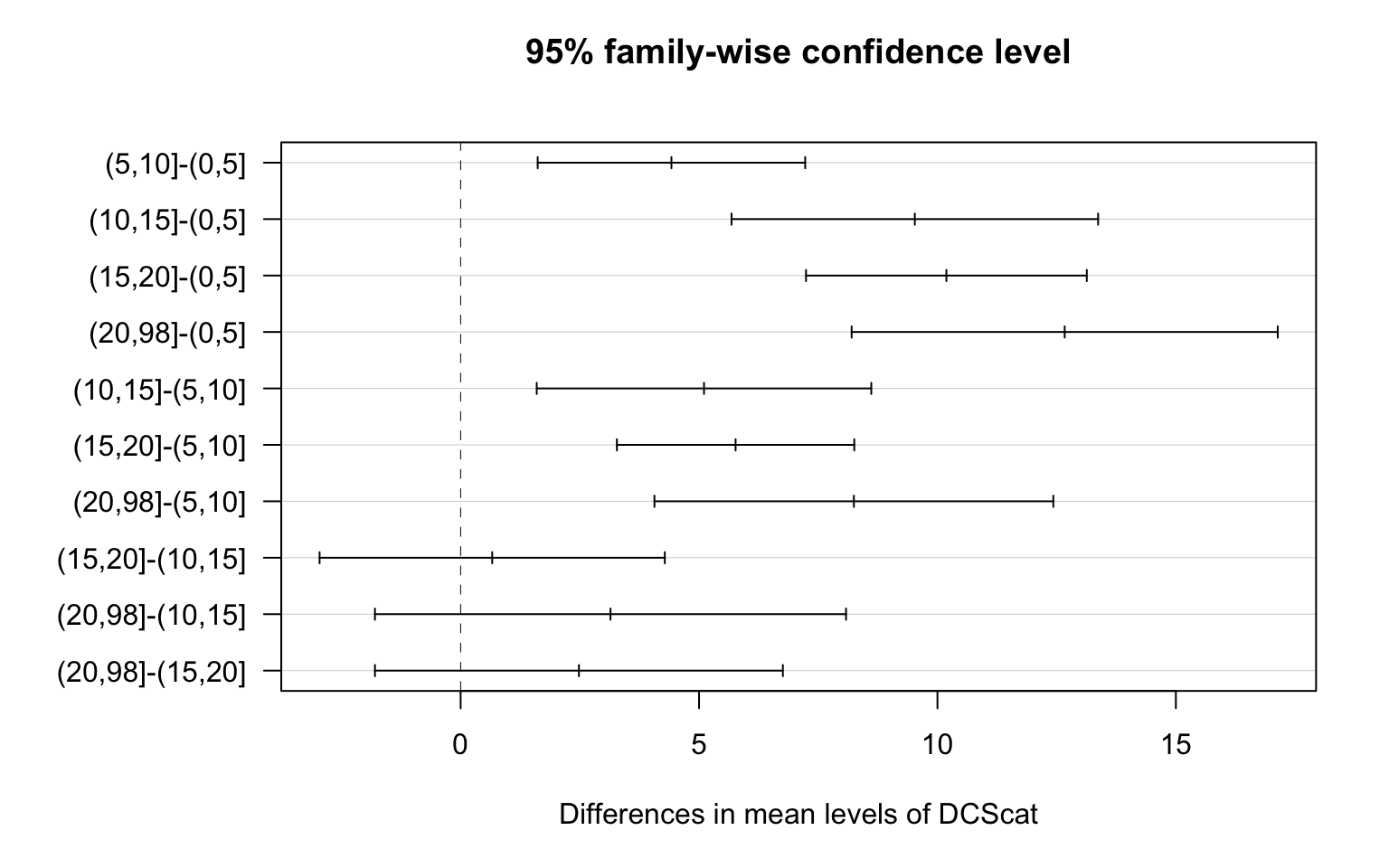
par(opar)ANOVA revealed that among daily, young adult smokers (my sample), number of cigarettes smoked per day (collapsed into 5 ordered categories, which is the categorical explanatory variable) and number of nicotine dependence symptoms (quantitative response variable) were significantly associated, F (4, 1310) = 31.95, p < 0.0001. Post hoc comparisons of mean number of nicotine dependence symptoms by pairs of cigarettes per day categories revealed that those individuals smoking more than 10 cigarettes per day (i.e. 11 to 15, 16 to 20 and >20) reported significantly more nicotine dependence symptoms compared to those smoking 10 or fewer cigarettes per day (i.e. 1 to 5 and 6 to 10 cigarettes per day).