One Qualitative Predictor

Author

Most material from Probability and Statistics with R, Second Edition

Published

Last modified on September 17, 2024 08:54:45 Eastern Daylight Time

Qualitative Predictors

The simplest situation where dummy variables might be used in a regression model is when the qualitative predictor has only two levels. The regression model for a single quantitative predictor \((x_1)\) and a dummy variable \((D_1)\) is written

\[\begin{equation} Y = \beta_0 + \beta_1 x_1 + \beta_2 D_1 + \beta_3 x_1 D_1 + \varepsilon \end{equation}\] where \[\begin{equation*} D_1 = \begin{cases} 0 &\text{for the first level}\\ 1 &\text{for the second level.} \end{cases} \end{equation*}\]

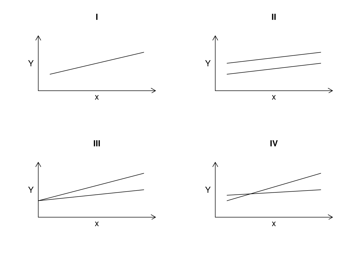
The model above when \(D_1\) has two levels will yield one of four possible scenarios, as shown in Figure 1. This type of model requires the user to answer three basic questions:

  • Are the lines the same?
  • Are the slopes the same?
  • Are the intercepts the same?

Figure 1: Four possible results for a single dummy variable with two levels. Graph I has the intercept and the slope the same for both levels of the dummy variable. Graph II has the two lines with the same slope, but different intercepts. Graph III shows the two fitted lines with the same intercept but different slopes. Graph IV shows the two lines with different intercepts and different slopes.

To address whether the lines are the same, the null hypothesis \(H_0: \beta_2 = \beta_3 = 0\) must be tested. One way to perform the test is to use the general linear test statistic based on the full model and the reduced model \(Y = \beta_0 + \beta_1 x_1 + \varepsilon\). If the null hypothesis is not rejected, the interpretation is that there is one line present (the intercept and the slope are the same for both levels of the dummy variable). This is the case for graph I of Figure 1. If the null hypothesis is rejected, either the slopes, the intercepts, or possibly both the slope and the intercept are different for the different levels of the dummy variable, as seen in graphs II, III, and IV of Figure 1, respectively.

To answer whether the slopes are the same, the null hypothesis \(H_0: \beta_3 = 0\) must be tested. If the null hypothesis is not rejected, the two lines have the same slope, but different intercepts, as shown in graph II of Figure 1. The two parallel lines that result when \(\beta_3 = 0\) are

\[\begin{equation*} Y = \beta_0 + \beta_1 x_1 + \varepsilon \text{ for } (D_1 = 0) \quad\text{and}\quad Y = (\beta_0 +\beta_2) + \beta_1 x_1 + \varepsilon \text{ for } (D_1 = 1). \end{equation*}\]

When \(H_0: \beta_3=0\) is rejected, one concludes that the two fitted lines are not parallel as in graphs III and IV of Figure 1.

To answer whether the intercepts are the same, the null hypothesis \(H_0: \beta_2 = 0\) for the full model must be tested. The reduced model for this test is \(Y = \beta_0 + \beta_1 x_1 + \beta_3 x_1 D_1 + \varepsilon\). If the null hypothesis is not rejected, the two fitted lines have the same intercept but different slopes:

\[\begin{equation*} Y = \beta_0 + \beta_1 x_1 + \varepsilon \text{ for } (D_1 = 0) \quad\text{and}\quad Y = \beta_0 + (\beta_1 +\beta_3) x_1 + \varepsilon \text{ for } (D_1 = 1). \end{equation*}\]

Graph III of Figure 1 represents this situation. If the null hypothesis is rejected, one concludes that the two lines have different intercepts, as in graphs II and IV of Figure 1.

Example

Suppose a realtor wants to model the appraised price of an apartment as a function of the predictors living area (in m\(^2\)) and the presence or absence of elevators. Consider the data frameVIT2005, which contains data about apartments in Vitoria, Spain, including totalprice, area, and elevator, which are the appraised apartment value in Euros, living space in square meters, and the absence or presence of at least one elevator in the building, respectively. The realtor first wants to know if there is any relationship between appraised price \((Y)\) and living area \((x_1)\). Next, the realtor wants to know how adding a dummy variable for whether or not an elevator is present changes the relationship: Are the lines the same? Are the slopes the same? Are the intercepts the same?

Solution (is there a realationship between totalprice and area?):

R Code
Code
library(tidyverse)
library(PASWR2)
VIT2005 <- VIT2005 |> 
  mutate(elevator = factor(elevator, labels = c("No", "Yes")))
mod_simple <- lm(totalprice ~ area, data = VIT2005)
summary(mod_simple) 

Call:
lm(formula = totalprice ~ area, data = VIT2005)

Residuals:
    Min      1Q  Median      3Q     Max 
-156126  -21564   -2155   19493  120674 

Coefficients:
            Estimate Std. Error t value Pr(>|t|)    
(Intercept)  40822.4    12170.1   3.354  0.00094 ***
area          2704.8      133.6  20.243  < 2e-16 ***
---
Signif. codes:  0 '***' 0.001 '**' 0.01 '*' 0.05 '.' 0.1 ' ' 1

Residual standard error: 40810 on 216 degrees of freedom
Multiple R-squared:  0.6548,    Adjusted R-squared:  0.6532 
F-statistic: 409.8 on 1 and 216 DF,  p-value: < 2.2e-16
Code
library(moderndive)
get_regression_table(mod_simple) |> 
  kable()
term estimate std_error statistic p_value lower_ci upper_ci
intercept 40822.416 12170.092 3.354 0.001 16835.075 64809.757
area 2704.751 133.616 20.243 0.000 2441.393 2968.109
Code
ggplot(data = VIT2005, aes(x = area, y = totalprice)) +
  geom_point() +
  theme_bw() +
  geom_smooth(method = "lm", se = FALSE) +
  scale_y_continuous(labels = label_currency(prefix = "€")) +
  scale_x_continuous(labels = label_number(suffix = " square meters")) +
  labs(x = "Apartment Area", y = "Appraised Price")

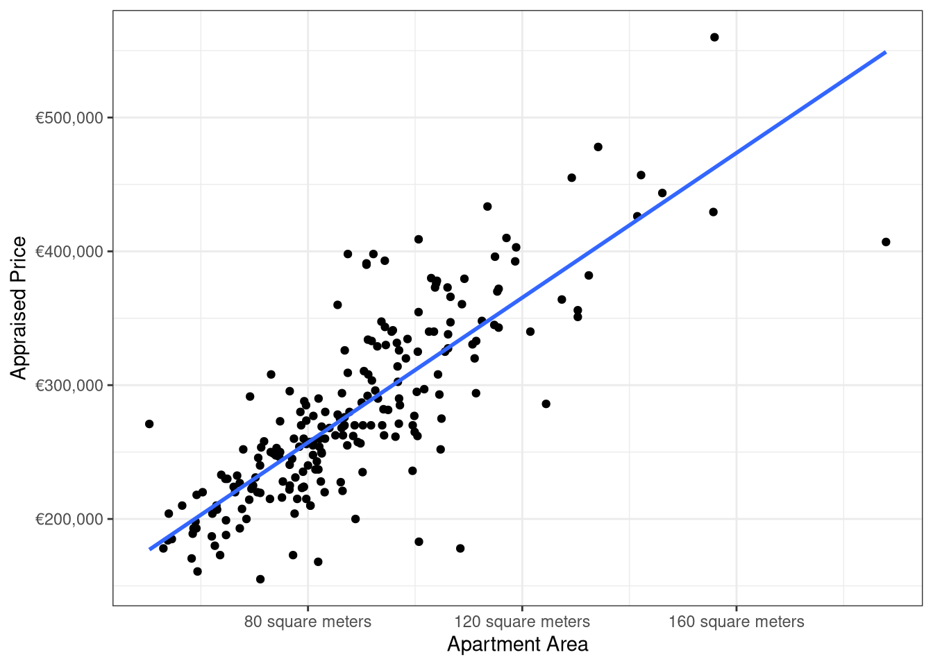
Figure 2: Scatterplot of totalprice versus area with the fitted regression line superimposed from mod_simple

A linear regression model of the form

\[\begin{equation} Y= \beta_0 +\beta_1 x_1 + \varepsilon \end{equation}\]

is fit yielding

\[\begin{equation*} \widehat{Y}_i = 40,822 + 2,705 x_{i1} \end{equation*}\]

and a scatterplot of totalprice versus area with the fitted regression line superimposed over the scatterplot is shown in Figure 2.

Based on Figure 2, there appears to be a linear relationship between appraised price and living area. Further, this relationship is statistically significant, as the p-value for testing \(H_0: \beta_1=0\) versus \(H_1: \beta_1 \neq 0\) is less than \(2 \times 10^{-16}\).

Solution (does adding a dummy variable (elevator) change the relationship?):

The regression model including the dummy variable for elevator is written \[\begin{equation} Y = \beta_0 + \beta_1 x_1 + \beta_2 D_1 + \beta_3 x_1 D_1 + \varepsilon \end{equation}\] where \[\begin{equation*} D_1 = \begin{cases} 0 &\text{when a building has no elevators}\\ 1 &\text{when a building has at least one elevator.} \end{cases} \end{equation*}\]

To determine if the lines are the same (which means that the linear relationship between appraised price and living area is the same for apartments with and without elevators), the hypotheses are

\[\begin{equation*} H_0: \beta_2 = \beta_3 = 0 \text{ versus } H_1: \text{at least one } \beta_i \neq 0 \text{ for } i=2, 3. \end{equation*}\]
R Code
Code
mod_full <- lm(totalprice ~ area + elevator + area:elevator, data = VIT2005)
anova(mod_simple, mod_full)  # compare models
Analysis of Variance Table

Model 1: totalprice ~ area
Model 2: totalprice ~ area + elevator + area:elevator
  Res.Df        RSS Df Sum of Sq      F    Pr(>F)    
1    216 3.5970e+11                                  
2    214 3.0267e+11  2 5.704e+10 20.165 9.478e-09 ***
---
Signif. codes:  0 '***' 0.001 '**' 0.01 '*' 0.05 '.' 0.1 ' ' 1

In this problem, one may conclude that at least one of \(\beta_2\) and \(\beta_3\) is not zero since the p-value = \(9.4780144\times 10^{-9}\). In other words, the lines have either different intercepts, different slopes, or different intercepts and slopes.

To see if the lines have the same slopes (which means that the presence of an elevator adds constant value over all possible living areas), the hypotheses are \[\begin{equation*} H_0: \beta_3 = 0 \text{ versus } H_1: \beta_3 \neq 0. \end{equation*}\]

R Code
Code
anova(mod_full)
Analysis of Variance Table

Response: totalprice
               Df     Sum Sq    Mean Sq  F value    Pr(>F)    
area            1 6.8239e+11 6.8239e+11 482.4846 < 2.2e-16 ***
elevator        1 4.5308e+10 4.5308e+10  32.0352  4.83e-08 ***
area:elevator   1 1.1732e+10 1.1732e+10   8.2949   0.00438 ** 
Residuals     214 3.0267e+11 1.4143e+09                       
---
Signif. codes:  0 '***' 0.001 '**' 0.01 '*' 0.05 '.' 0.1 ' ' 1

Based on the p-value = \(0.0043797\), it may be concluded that \(\beta_3 \neq 0\), which implies that the lines are not parallel.

To test for equal intercepts (which means that appraised price with and without elevators starts at the same value), the hypotheses to be evaluated are \[\begin{equation*} H_0: \beta_2 = 0 \text{ versus }H_1: \beta_2 \neq 0. \end{equation*}\]

R Code
Code
mod_full <- lm(totalprice ~ area + elevator + area:elevator, data = VIT2005)
mod_inter <- lm(totalprice ~ area + area:elevator, data = VIT2005)
# compare models
anova(mod_inter, mod_full) 
Analysis of Variance Table

Model 1: totalprice ~ area + area:elevator
Model 2: totalprice ~ area + elevator + area:elevator
  Res.Df        RSS Df  Sum of Sq      F Pr(>F)
1    215 3.0624e+11                            
2    214 3.0267e+11  1 3576497188 2.5288 0.1133

Since the p-value for testing the null hypothesis is 0.1132635, one fails to reject \(H_0\) and should conclude that the two lines have the same intercept but different slopes.

R Code
Code
summary(mod_inter)

Call:
lm(formula = totalprice ~ area + area:elevator, data = VIT2005)

Residuals:
    Min      1Q  Median      3Q     Max 
-125093  -21762   -2201   18117  112252 

Coefficients:
                 Estimate Std. Error t value Pr(>|t|)    
(Intercept)      71352.08   12309.18   5.797 2.39e-08 ***
area              1897.94     180.59  10.510  < 2e-16 ***
area:elevatorYes   553.99      90.42   6.127 4.23e-09 ***
---
Signif. codes:  0 '***' 0.001 '**' 0.01 '*' 0.05 '.' 0.1 ' ' 1

Residual standard error: 37740 on 215 degrees of freedom
Multiple R-squared:  0.7061,    Adjusted R-squared:  0.7034 
F-statistic: 258.3 on 2 and 215 DF,  p-value: < 2.2e-16
Code
coef(mod_inter)
     (Intercept)             area area:elevatorYes 
      71352.0844        1897.9368         553.9856 
Code
b0 <- coef(mod_inter)[1]
b1NO <- coef(mod_inter)[2]
b1YES <- coef(mod_inter)[2] + coef(mod_inter)[3]
c(b0, b1NO, b1YES)
(Intercept)        area        area 
  71352.084    1897.937    2451.922 

The fitted model is \(\widehat{Y}_i = 71,352 + 1,898x_{i1} + 554x_{i1}D_{i1}\), and the fitted regression lines for the two values of \(D_1\) are shown in Figure 3. The fitted model using the same intercept with different slopes has an \(R^2_a\) of 0.7033949, a modest improvement over the model without the variable elevator, which had an \(R^2_a\) value of 0.6532269.

Code
ggplot(data = VIT2005, aes(x = area, y = totalprice, color = elevator)) +
  geom_point(alpha = 0.5) +
  theme_bw() +
  geom_abline(intercept = b0,
              slope = b1NO,
              color = "red") +
  geom_abline(intercept = b0,
              slope = b1YES,
              color = "blue") +
  scale_color_manual(values = c("red", "blue")) +
  labs(x = "Apartment Area", 
       y = "Appraised Price",
       color = "Elevator") +
  scale_y_continuous(labels = label_currency(prefix = "€"),
                     limits = c(50000, 500000)) +
  scale_x_continuous(labels = label_number(suffix = " square meters"),
                     limits = c(10, 200)) 
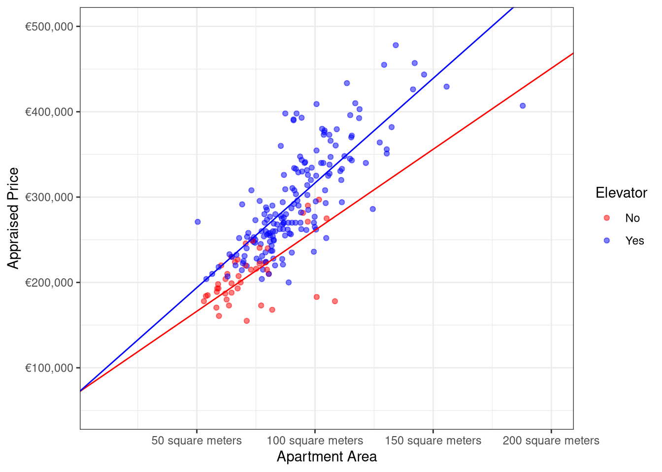
Figure 3: Fitted regression lines for mod_inter

Diagnostics

R Code
Code
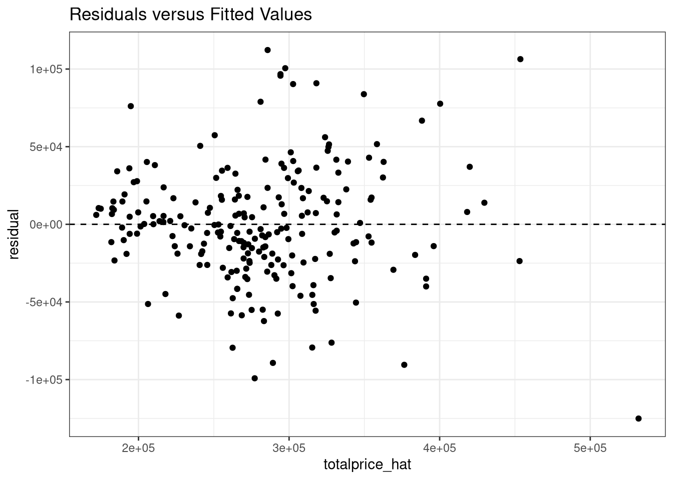
MDF <- get_regression_points(mod_inter)
ggplot(data = MDF, aes(x = totalprice_hat, y = residual)) +
  geom_point() +
  theme_bw() +
  labs(title = "Residuals versus Fitted Values") +
  geom_hline(yintercept = 0, lty = "dashed")

Code
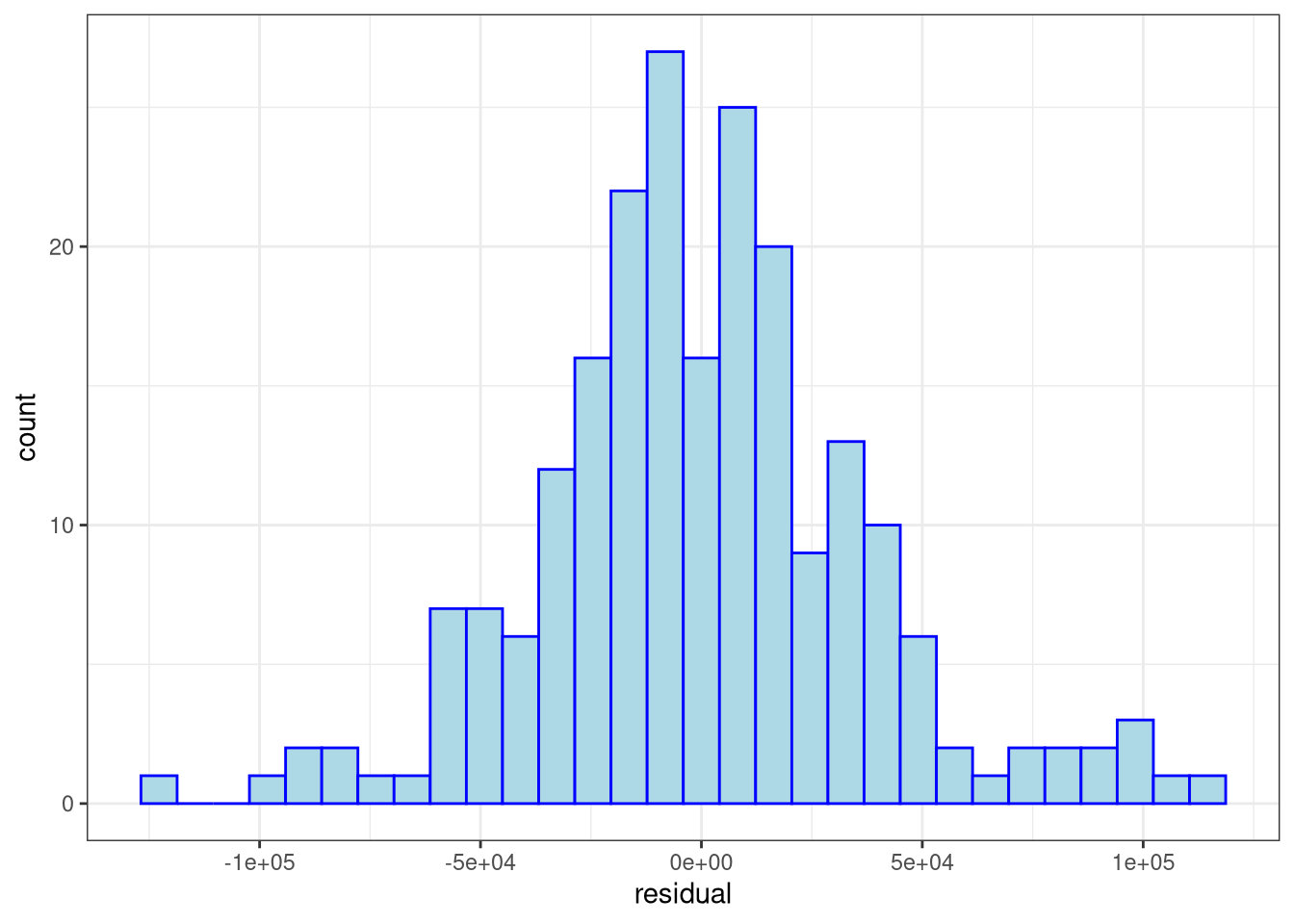
ggplot(data = MDF, aes(x = residual)) +
  geom_histogram(fill = "lightblue", color = "blue") +
  theme_bw() 

Code
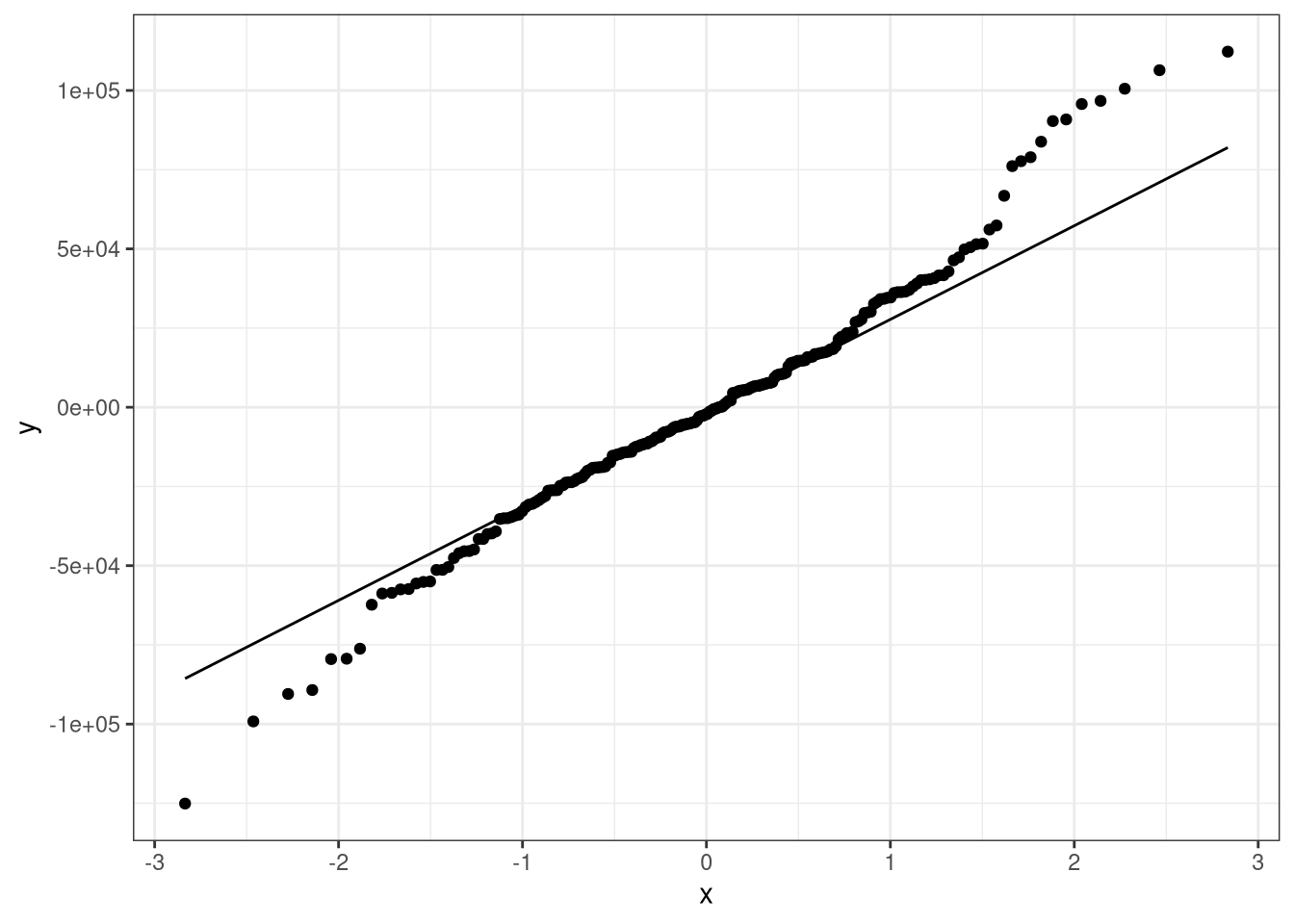
ggplot(data = MDF, aes(sample = residual)) +
  geom_qq() +
  geom_qq_line() +
  theme_bw() 


Example

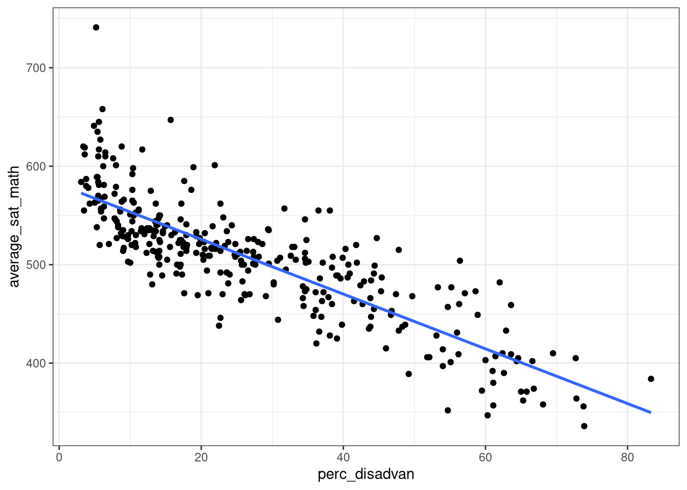
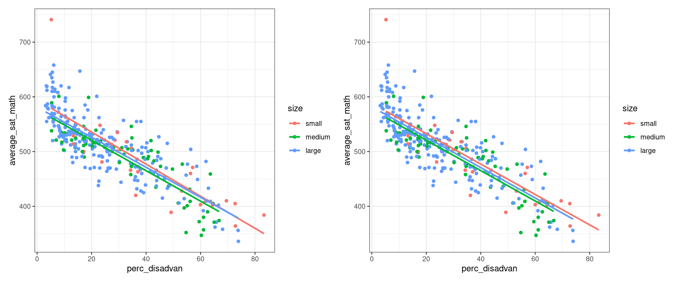
Consider the MA_schools data frame from the moderndive package which contains 2017 data on Massachusetts public high schools provided by the Massachusetts Department of Education. Consider a model with SAT math scores (average_sat_math) modeled as a function of percentage of the high school’s student body that are economically disadvantaged (perc_disadvan) and the a categorical variable measuring school size (size).

Solution (is there a relationship between average_sat_math and perc_disadvan?):

R Code
Code
ggplot(data = MA_schools, 
       aes(x = perc_disadvan, y = average_sat_math)) + 
  geom_point() +
  theme_bw() + 
  geom_smooth(method = "lm", se = FALSE)

Code
mod_simple <- lm(average_sat_math ~ perc_disadvan, 
                 data = MA_schools)
summary(mod_simple)

Call:
lm(formula = average_sat_math ~ perc_disadvan, data = MA_schools)

Residuals:
   Min     1Q Median     3Q    Max 
-80.74 -21.26  -4.12  18.54 174.17 

Coefficients:
              Estimate Std. Error t value Pr(>|t|)    
(Intercept)   581.2811     3.2668   177.9   <2e-16 ***
perc_disadvan  -2.7798     0.1011   -27.5   <2e-16 ***
---
Signif. codes:  0 '***' 0.001 '**' 0.01 '*' 0.05 '.' 0.1 ' ' 1

Residual standard error: 33.54 on 330 degrees of freedom
Multiple R-squared:  0.6962,    Adjusted R-squared:  0.6953 
F-statistic: 756.2 on 1 and 330 DF,  p-value: < 2.2e-16
Code
get_regression_table(mod_simple) |> 
  kable()
term estimate std_error statistic p_value lower_ci upper_ci
intercept 581.281 3.267 177.936 0 574.855 587.707
perc_disadvan -2.780 0.101 -27.499 0 -2.979 -2.581

You complete the rest….

Solution (does adding a dummy variable size change the relationship?):

R Code
Code
ggplot(data = MA_schools, 
       aes(x = perc_disadvan, y = average_sat_math, color = size)) + 
  geom_point() +
  theme_bw() + 
  geom_smooth(method = "lm", se = FALSE) -> p1
ggplot(data = MA_schools, 
       aes(x = perc_disadvan, y = average_sat_math, color = size)) + 
  geom_point() +
  theme_bw() + 
  geom_parallel_slopes(se = FALSE) -> p2
library(patchwork)
p1 + p2

Code
mod_full <- lm(lm(average_sat_math ~ perc_disadvan + size + perc_disadvan:size, data = MA_schools))
anova(mod_simple, mod_full) |> 
  kable()
Res.Df RSS Df Sum of Sq F Pr(>F)
330 371190.9 NA NA NA NA
326 367669.4 4 3521.459 0.7805895 0.5384385
Code
anova(mod_full) |> 
  kable()
Df Sum Sq Mean Sq F value Pr(>F)
perc_disadvan 1 850614.7701 850614.7701 754.2112099 0.0000000
size 2 3132.6259 1566.3130 1.3887965 0.2508467
perc_disadvan:size 2 388.8332 194.4166 0.1723826 0.8417338
Residuals 326 367669.4425 1127.8204 NA NA

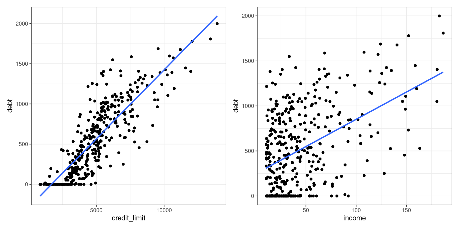
Simpson’s Paradox

R Code
Code
library(ISLR)
credit_paradox <- Credit |> 
  select(ID, debt = Balance, credit_limit = Limit, 
         credit_rating = Rating, income = Income, age = Age)
ggplot(data = credit_paradox, aes(x = credit_limit, y = debt)) + 
  geom_point() + 
  geom_smooth(method = "lm", se = FALSE) + 
  theme_bw() -> p1
ggplot(data = credit_paradox, aes(x = income, y = debt)) + 
  geom_point() + 
  geom_smooth(method = "lm", se = FALSE) + 
  theme_bw() -> p2
library(patchwork)
p1 + p2

Code
library(plotly)
p <- plot_ly(data = credit_paradox, z = ~debt, x = ~credit_limit, y = ~income) |> 
  add_markers()
p
Code
mod <- lm(debt ~ credit_limit + income, data = credit_paradox)
summary(mod)$coef
                 Estimate   Std. Error   t value      Pr(>|t|)
(Intercept)  -385.1792604 19.464801525 -19.78850  3.878764e-61
credit_limit    0.2643216  0.005879729  44.95471 7.717386e-158
income         -7.6633230  0.385072058 -19.90101  1.260933e-61
Code
x <- seq(min(credit_paradox$credit_limit), max(credit_paradox$credit_limit), length = 70)
y <- seq(min(credit_paradox$income), max(credit_paradox$income), length = 70) 
plane <- outer(x, y, function(a, b){coef(mod)[1] + coef(mod)[2]*a + coef(mod)[3]*b})
# draw the plane
p |> 
  add_surface(x = ~x, y = ~y, z = ~plane)
Code
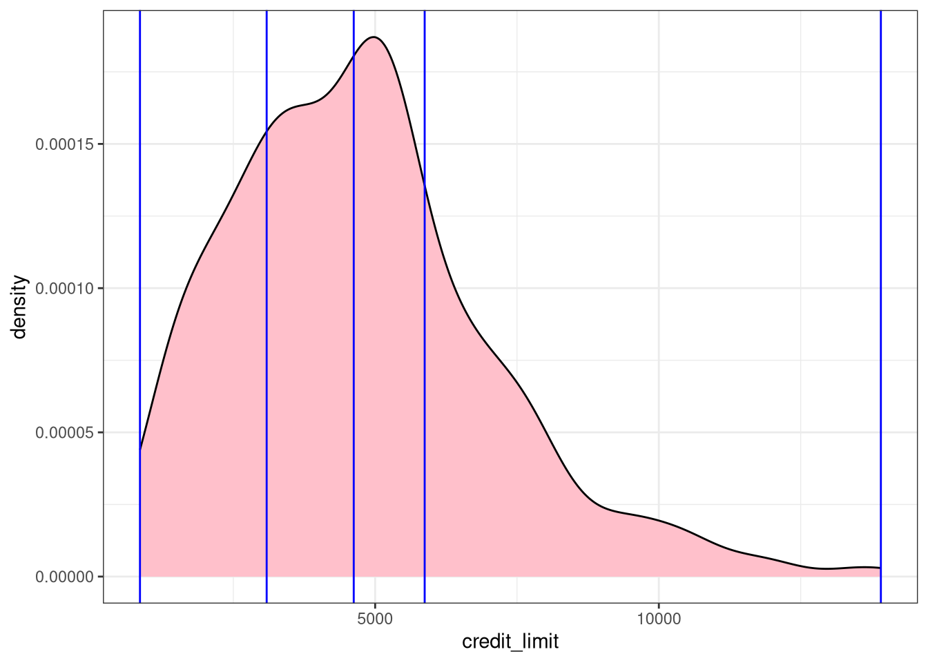
qs <- quantile(credit_paradox$credit_limit, probs = seq(0, 1, .25))
# credit_paradox$credit_cats <- cut(credit_paradox$credit_limit, breaks = qs, include.lowest = TRUE)
############### Or above
credit_paradox <- credit_paradox |> 
  mutate(credit_cats = cut(credit_limit, breaks = qs, include.lowest = TRUE))
head(credit_paradox)
  ID debt credit_limit credit_rating  income age         credit_cats
1  1  333         3606           283  14.891  34 (3.09e+03,4.62e+03]
2  2  903         6645           483 106.025  82 (5.87e+03,1.39e+04]
3  3  580         7075           514 104.593  71 (5.87e+03,1.39e+04]
4  4  964         9504           681 148.924  36 (5.87e+03,1.39e+04]
5  5  331         4897           357  55.882  68 (4.62e+03,5.87e+03]
6  6 1151         8047           569  80.180  77 (5.87e+03,1.39e+04]
Code
ggplot(data = credit_paradox, aes(x = credit_limit)) +
  geom_density(fill = "pink", color = "black") + 
  geom_vline(xintercept = qs, color = "blue") + 
  theme_bw()

Code
credit_paradox |> 
  group_by(credit_cats) |> 
  summarize(n())
# A tibble: 4 × 2
  credit_cats         `n()`
  <fct>               <int>
1 [855,3.09e+03]        100
2 (3.09e+03,4.62e+03]   100
3 (4.62e+03,5.87e+03]   100
4 (5.87e+03,1.39e+04]   100
Code
p1 <- ggplot(data = credit_paradox, aes(x = income, y = debt)) + 
  geom_point() +
  geom_smooth(method = "lm", se = FALSE) + 
  theme_bw() + 
  labs(y = "Credit card debt (in $)",
       x = "Income (in $1000)")
p2 <- ggplot(data = credit_paradox, aes(x = income, y = debt, color = credit_cats)) + 
  geom_point() +
  geom_smooth(method = "lm", se = FALSE) + 
  theme_bw() + 
  labs(y = "Credit card debt (in $)",
       x = "Income (in $1000)",
       color = "Credit limit bracket")
p1 + p2

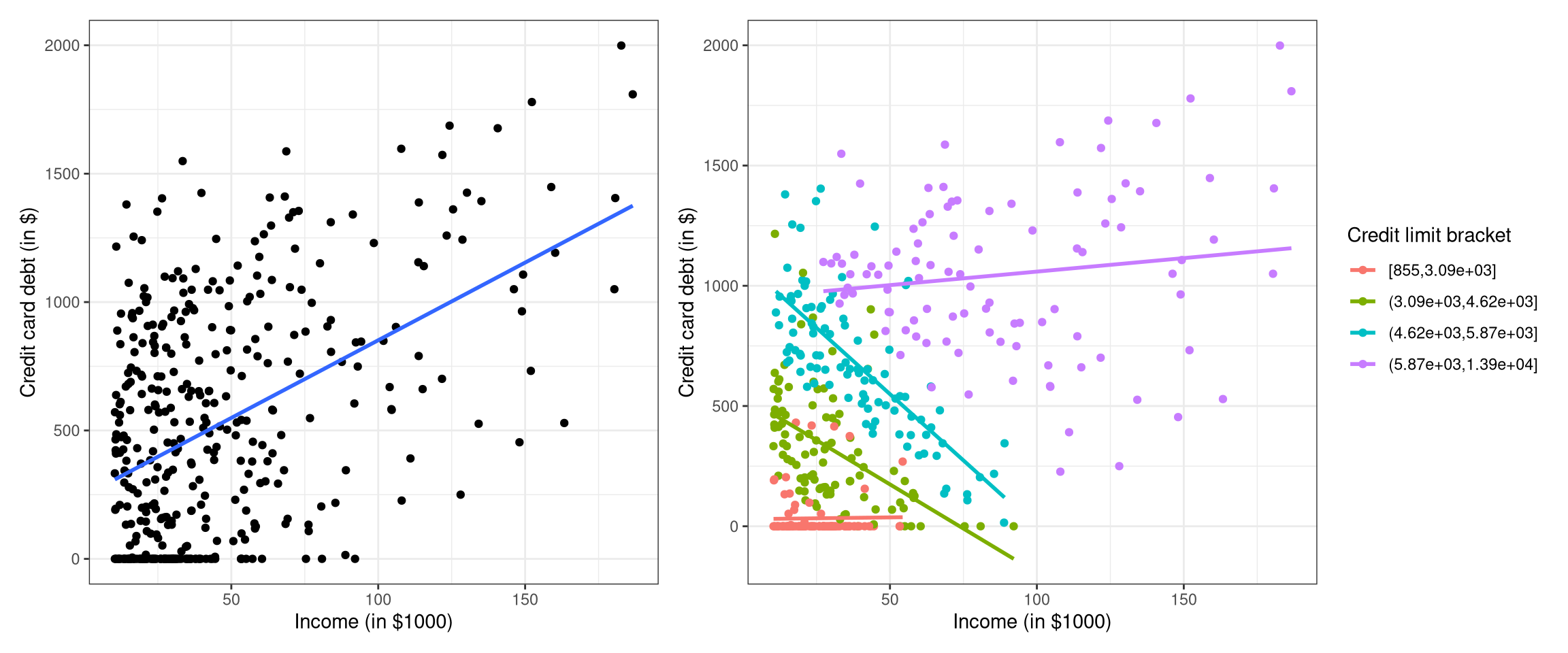
Relationship between credit card debt and income by credit limit bracket