One Categorical Variable - Hints

Author

ATA - In-class

Published

Last modified on September 15, 2026 12:09:52 Eastern Daylight Time

Exploratory Data Analysis

R Code

Code

library(gapminder)
gapminder1982 <- gapminder |> 
  filter(year == 1982) |> 
  rename(lifeexp = lifeExp, gdppercap = gdpPercap) |> 
  select(country, lifeexp, continent, gdppercap) 
gapminder1982 |> 
  head() |> 
  kable()

country	lifeexp	continent	gdppercap
Afghanistan	39.854	Asia	978.0114
Albania	70.420	Europe	3630.8807
Algeria	61.368	Africa	5745.1602
Angola	39.942	Africa	2756.9537
Argentina	69.942	Americas	8997.8974
Australia	74.740	Oceania	19477.0093

Code

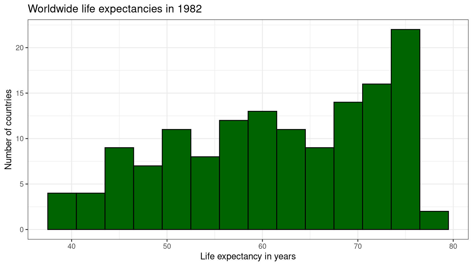
```{r}
#| label: "fig-exp"
#| fig-cap: "Worldwide life expectancies in 1982"
ggplot(data = gapminder1982, aes(x = lifeexp)) +
  geom_histogram(binwidth = 3,
                 color = "black",
                 fill = "darkgreen") +
  theme_bw() +
  labs(title = "Worldwide life expectancies in 1982",
       x = "Life expectancy in years",
       y = "Number of countries")
```

Figure 1: Worldwide life expectancies in 1982

Based on Figure 1, woldwide life expectancies in 1982 has a unimodal skew left distribution with statistics given in Table 1.

Code

```{r}
#| label: "tbl-stat"
#| tbl-cap: "Descriptive statistics" 
library(e1071)
gapminder1982 |> 
  summarize(
    Median = median(lifeexp),
    IQR = IQR(lifeexp),
    Skew = skewness(lifeexp)
  ) -> T1
T1 |> 
  knitr::kable()
```

Table 1: Descriptive statistics

Median	IQR	Skew
62.4415	17.98125	-0.3427068

Code

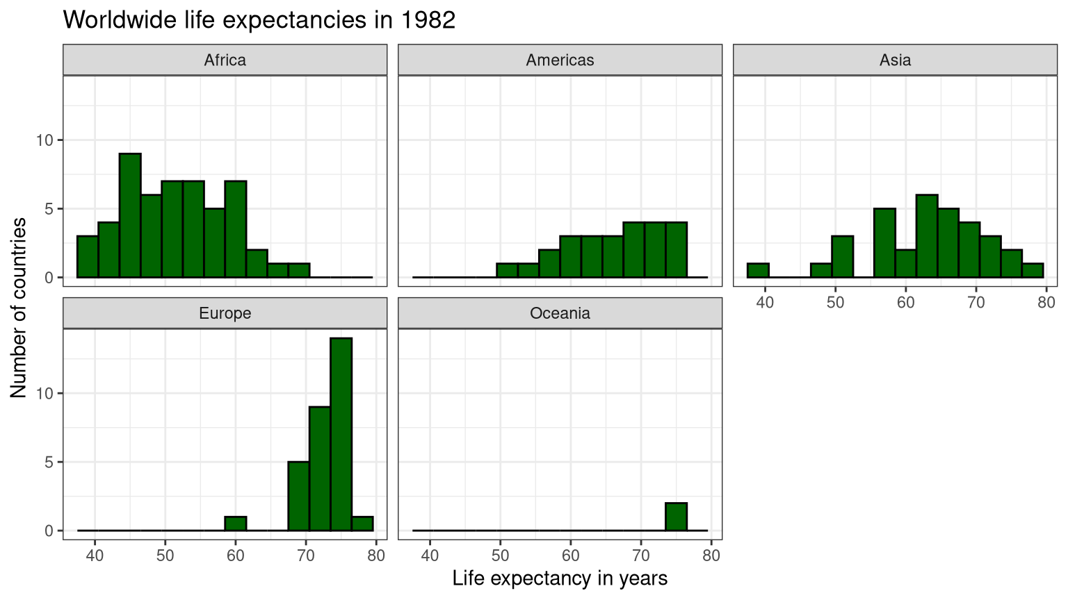
ggplot(data = gapminder1982, aes(x = lifeexp)) +
  geom_histogram(binwidth = 3,
                 color = "black",
                 fill = "darkgreen") +
  theme_bw() +
  labs(title = "Worldwide life expectancies in 1982",
       x = "Life expectancy in years",
       y = "Number of countries") +
  facet_wrap(vars(continent))

Code

gapminder1982 |>
  group_by(continent) |>
  summarize(
    Mean = mean(lifeexp),
    SD = sd(lifeexp),
    Median = median(lifeexp),
    IQR = IQR(lifeexp)
  ) -> results
results |> 
  knitr::kable()

Table 2: Statistics by continent

continent	Mean	SD	Median	IQR
Africa	51.59287	7.3759401	50.756	10.97025
Americas	66.22884	6.7208338	67.405	9.39900
Asia	62.61794	8.5352214	63.739	11.26800
Europe	72.80640	3.2182603	73.490	4.11750
Oceania	74.29000	0.6363961	74.290	0.45000

Code

lifeexp_mod <- lm(lifeexp ~ continent, data = gapminder1982)
get_regression_table(lifeexp_mod) -> T2
T2 |> 
  knitr::kable()

term	estimate	std_error	statistic	lower_ci	upper_ci
intercept	51.593	0.955	54.051	49.705	53.480
continent: Americas	14.636	1.675	8.737	11.323	17.949
continent: Asia	11.025	1.532	7.197	7.996	14.054
continent: Europe	21.214	1.578	13.443	18.093	24.334
continent: Oceania	22.697	4.960	4.576	12.889	32.505

Code

#OR
T2 |> 
  gt::gt()

term	estimate	std_error	statistic	lower_ci	upper_ci
intercept	51.593	0.955	54.051	49.705	53.480
continent: Americas	14.636	1.675	8.737	11.323	17.949
continent: Asia	11.025	1.532	7.197	7.996	14.054
continent: Europe	21.214	1.578	13.443	18.093	24.334
continent: Oceania	22.697	4.960	4.576	12.889	32.505

Report the average life expectancy for Africans in 1982 using lifeexp_mod.

Code

T2[1, "estimate"] |> pull()

[1] 51.593

Code

T2[1, 2] |> pull()

[1] 51.593

Code

coef(lifeexp_mod)[1]

(Intercept) 
   51.59287

The average life expectancy for Africans in 1982 was 51.593 years. Or, one could use coef(lifeexp_mod)[1] to return 51.5928654 years.

Report the average life expectancy for Europeans in 1982 using lifeexp_mod.

Code

T2[1,2] |> pull() + T2[4,2] |> pull()

[1] 72.807

Code

coef(lifeexp_mod)[1] + coef(lifeexp_mod)[4]

(Intercept) 
    72.8064

Code

round(coef(lifeexp_mod)[1] + coef(lifeexp_mod)[4],3)

(Intercept) 
     72.806

Code

predict(lifeexp_mod, newdata = data.frame(continent = "Europe"))

      1 
72.8064

The average life expectancy for Europeans in 1982 was 72.807 years.

Note: moderndive wrapper functions round answers. This is not always a good thing. It is best to leave the rounding until the very end! Consider the following inline R code.

The average life expectancy for Europeans in 1982 was 72.8064 years. Which if you want to round to three decimal places would be: 72.806 years. Another way to get the desired answer is with the predict() function. The average life expectancy for Europeans in 1982 was 72.8064 years.

Code

names(gapminder1982)

[1] "country"   "lifeexp"   "continent" "gdppercap"

Code

mod_full <- lm(lifeexp ~ gdppercap*continent, data = gapminder1982)

mod_simple <- lm(lifeexp ~ gdppercap + continent, data = gapminder1982)

anova(mod_simple, mod_full)

Analysis of Variance Table

Model 1: lifeexp ~ gdppercap + continent
Model 2: lifeexp ~ gdppercap * continent
  Res.Df    RSS Df Sum of Sq      F Pr(>F)
1    136 4811.7                           
2    132 4553.2  4    258.54 1.8738 0.1187

Code

anova(mod_full)

Analysis of Variance Table

Response: lifeexp
                     Df Sum Sq Mean Sq  F value    Pr(>F)    
gdppercap             1 8544.6  8544.6 247.7152 < 2.2e-16 ***
continent             4 3000.6   750.1  21.7472 8.411e-14 ***
gdppercap:continent   4  258.5    64.6   1.8738    0.1187    
Residuals           132 4553.2    34.5                       
---
Signif. codes:  0 '***' 0.001 '**' 0.01 '*' 0.05 '.' 0.1 ' ' 1

Code

modpar <- lm(lifeexp ~ gdppercap + continent, data = gapminder1982)
summary(modpar)


Call:
lm(formula = lifeexp ~ gdppercap + continent, data = gapminder1982)

Residuals:
     Min       1Q   Median       3Q      Max 
-18.9857  -3.0800  -0.0143   3.8538  16.6619 

Coefficients:
                   Estimate Std. Error t value Pr(>|t|)    
(Intercept)       5.014e+01  8.514e-01  58.894  < 2e-16 ***
gdppercap         5.852e-04  8.495e-05   6.889 1.91e-10 ***
continentAmericas 1.170e+01  1.509e+00   7.749 1.93e-12 ***
continentAsia     8.127e+00  1.389e+00   5.851 3.48e-08 ***
continentEurope   1.353e+01  1.762e+00   7.676 2.87e-12 ***
continentOceania  1.329e+01  4.498e+00   2.955  0.00369 ** 
---
Signif. codes:  0 '***' 0.001 '**' 0.01 '*' 0.05 '.' 0.1 ' ' 1

Residual standard error: 5.948 on 136 degrees of freedom
Multiple R-squared:  0.7058,    Adjusted R-squared:  0.695 
F-statistic: 65.26 on 5 and 136 DF,  p-value: < 2.2e-16

Code

library(moderndive)
get_regression_table(mod_simple) |> knitr::kable()

term	estimate	std_error	statistic	p_value	lower_ci	upper_ci
intercept	50.141	0.851	58.894	0.000	48.457	51.824
gdppercap	0.001	0.000	6.889	0.000	0.000	0.001
continent: Americas	11.695	1.509	7.749	0.000	8.711	14.680
continent: Asia	8.127	1.389	5.851	0.000	5.380	10.874
continent: Europe	13.526	1.762	7.676	0.000	10.041	17.011
continent: Oceania	13.291	4.498	2.955	0.004	4.395	22.187

Code

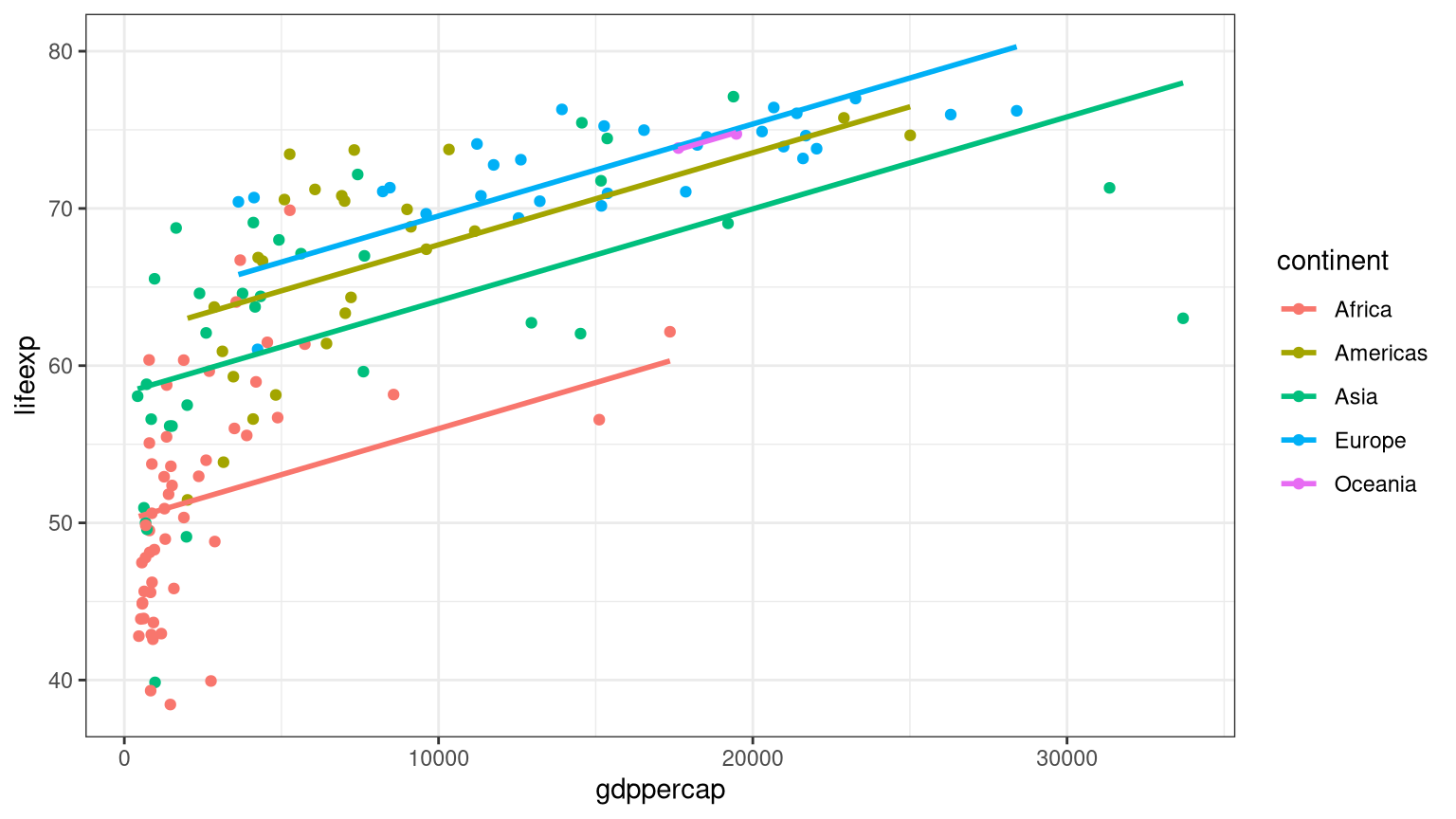
ggplot(data = gapminder1982, aes(x = gdppercap, y = lifeexp, color = continent)) + 
  geom_point() + 
  geom_parallel_slopes(se = FALSE) + 
  theme_bw()

Code

get_regression_table(mod_full) |>  knitr::kable()

term	estimate	std_error	statistic	p_value	lower_ci	upper_ci
intercept	48.759	1.029	47.371	0.000	46.723	50.795
gdppercap	0.001	0.000	4.503	0.000	0.001	0.002
continent: Americas	11.824	2.255	5.242	0.000	7.362	16.285
continent: Asia	9.952	1.700	5.852	0.000	6.588	13.316
continent: Europe	18.482	3.029	6.101	0.000	12.489	24.474
continent: Oceania	16.478	83.658	0.197	0.844	-149.005	181.961
gdppercap:continentAmericas	0.000	0.000	-1.168	0.245	-0.001	0.000
gdppercap:continentAsia	-0.001	0.000	-2.199	0.030	-0.001	0.000
gdppercap:continentEurope	-0.001	0.000	-2.578	0.011	-0.001	0.000
gdppercap:continentOceania	-0.001	0.005	-0.145	0.885	-0.010	0.008

Code

summary(mod_full)


Call:
lm(formula = lifeexp ~ gdppercap * continent, data = gapminder1982)

Residuals:
    Min      1Q  Median      3Q     Max 
-19.371  -3.292   0.000   3.222  15.111 

Coefficients:
                              Estimate Std. Error t value Pr(>|t|)    
(Intercept)                 48.7590520  1.0293042  47.371  < 2e-16 ***
gdppercap                    0.0011419  0.0002536   4.503 1.46e-05 ***
continentAmericas           11.8237096  2.2554654   5.242 6.13e-07 ***
continentAsia                9.9518599  1.7004659   5.852 3.63e-08 ***
continentEurope             18.4815305  3.0291958   6.101 1.09e-08 ***
continentOceania            16.4779018 83.6576503   0.197   0.8442    
gdppercap:continentAmericas -0.0003898  0.0003336  -1.168   0.2448    
gdppercap:continentAsia     -0.0006164  0.0002803  -2.199   0.0296 *  
gdppercap:continentEurope   -0.0007856  0.0003048  -2.578   0.0110 *  
gdppercap:continentOceania  -0.0006540  0.0045099  -0.145   0.8849    
---
Signif. codes:  0 '***' 0.001 '**' 0.01 '*' 0.05 '.' 0.1 ' ' 1

Residual standard error: 5.873 on 132 degrees of freedom
Multiple R-squared:  0.7216,    Adjusted R-squared:  0.7027 
F-statistic: 38.02 on 9 and 132 DF,  p-value: < 2.2e-16

Code

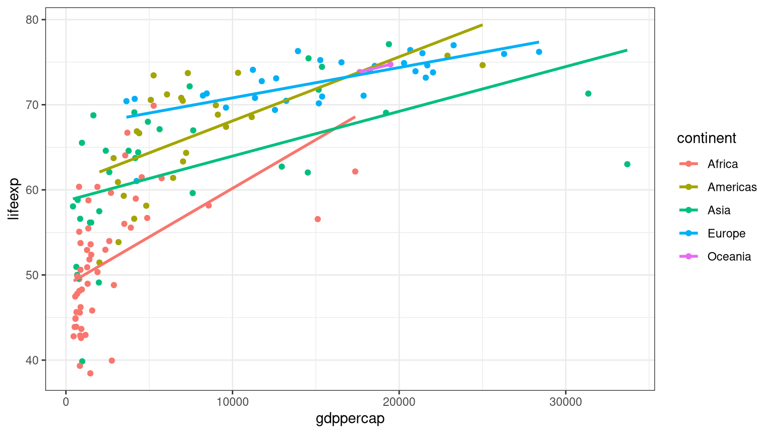
ggplot(data = gapminder1982, aes(x = gdppercap, y = lifeexp, color = continent)) + 
  geom_point() + 
  geom_smooth(method = "lm", se = FALSE) + 
  theme_bw()

Other Formats

Exploratory Data Analysis