Descriptive information and the appraised total price (in Euros) for apartments in Vitoria, Spain
VIT2005Format
A data frame with 218 observations on the following 5 variables:
totalprice(the market total price (in Euros) of the apartment including garage(s) and storage room(s))area(the total living area of the apartment in square meters)zone(a factor indicating the neighborhood where the apartment is located with levelsZ11,Z21,Z31,Z32,Z34,Z35,Z36,Z37,Z38,Z41,Z42,Z43,Z44,Z45,Z46,Z47,Z48,Z49,Z52,Z53,Z56,Z61, andZ62)category(a factor indicating the condition of the apartment with levels2A,2B,3A,3B,4A,4B, and5Aordered so that2Ais the best and5Ais the worst)age(age of the apartment in years)floor(floor on which the apartment is located)rooms(total number of rooms including bedrooms, dining room, and kitchen)out(a factor indicating the percent of the apartment exposed to the elements: The levelsE100,E75,E50, andE25, correspond to complete exposure, 75% exposure, 50% exposure, and 25% exposure, respectively.)conservation(is an ordered factor indicating the state of conservation of the apartment. The levels1A,2A,2B, and3Aare ordered from best to worst conservation.)toilets(the number of bathrooms)garage(the number of garages)elevator(indicates the absence (0) or presence (1) of elevators.)streetcategory(an ordered factor from best to worst indicating the category of the street with levelsS2,S3,S4, andS5)heating(a factor indicating the type of heating with levels1A,3A,3B, and4Awhich correspond to: no heating, low-standard private heating, high-standard private heating, and central heating, respectively.)storage(the number of storage rooms outside of the apartment)
References
Ugarte, M. D., Militino, A. F., and Arnholt, A. T. 2015. Probability and Statistics with R, Second Edition. Chapman & Hall / CRC.
Examples
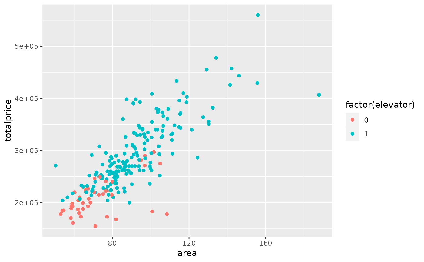
ggplot(data = VIT2005, aes(x = area, y = totalprice, color = factor(elevator))) +
geom_point()

modTotal <- lm(totalprice ~ area + as.factor(elevator) + area:as.factor(elevator),
data = VIT2005)
modSimpl <- lm(totalprice ~ area, data = VIT2005)
anova(modSimpl, modTotal)
#> Analysis of Variance Table
#>
#> Model 1: totalprice ~ area
#> Model 2: totalprice ~ area + as.factor(elevator) + area:as.factor(elevator)
#>   Res.Df        RSS Df Sum of Sq      F    Pr(>F)
#> 1    216 3.5970e+11
#> 2    214 3.0267e+11  2 5.704e+10 20.165 9.478e-09 ***
#> ---
#> Signif. codes:  0 ‘***’ 0.001 ‘**’ 0.01 ‘*’ 0.05 ‘.’ 0.1 ‘ ’ 1
rm(modSimpl, modTotal)
modTotal <- lm(totalprice ~ area + as.factor(elevator) + area:as.factor(elevator),
data = VIT2005)
modSimpl <- lm(totalprice ~ area, data = VIT2005)
anova(modSimpl, modTotal)
#> Analysis of Variance Table
#>
#> Model 1: totalprice ~ area
#> Model 2: totalprice ~ area + as.factor(elevator) + area:as.factor(elevator)
#> Res.Df RSS Df Sum of Sq F Pr(>F)
#> 1 216 3.5970e+11
#> 2 214 3.0267e+11 2 5.704e+10 20.165 9.478e-09 ***
#> ---
#> Signif. codes: 0 ‘***’ 0.001 ‘**’ 0.01 ‘*’ 0.05 ‘.’ 0.1 ‘ ’ 1
rm(modSimpl, modTotal)