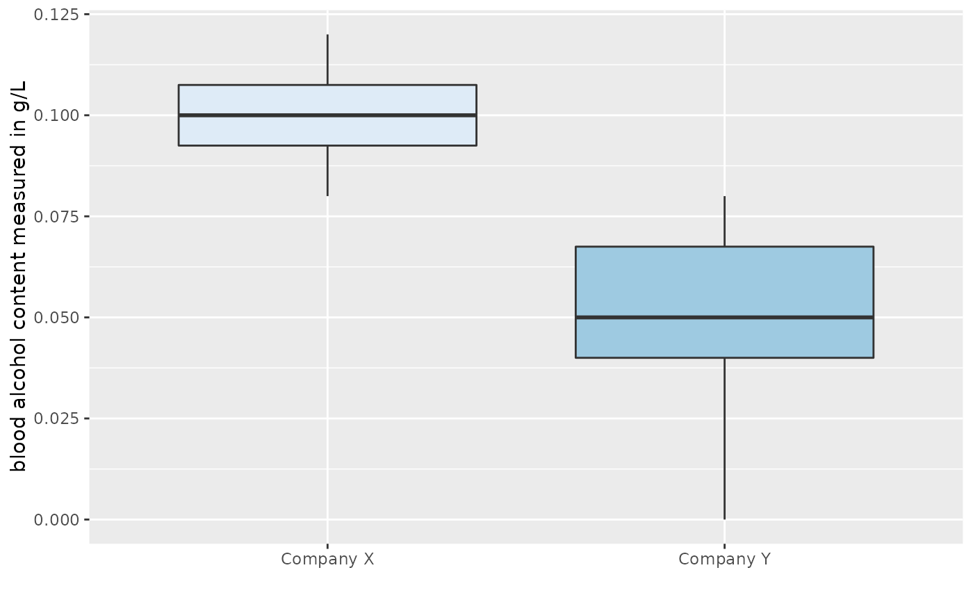
Two volunteers weighing 180 pounds each consumed a twelve ounce beer every fifteen minutes for one hour. One hour after the fourth beer was consumed, each volunteer's blood alcohol was measured with ten different breathalyzers from the same company. The numbers recorded in data frame BAC are the sorted blood alcohol content values reported with breathalyzers from company X and company Y.
BACFormat
A data frame with 10 observations of the following 2 variables:
X(blood alcohol content measured in g/L)Y(blood alcohol content measured in g/L)
References
Ugarte, M. D., Militino, A. F., and Arnholt, A. T. 2015. Probability and Statistics with R, Second Edition. Chapman & Hall / CRC.
Examples
with(data = BAC,
var.test(X, Y, alternative = "less"))
#>
#> 	F test to compare two variances
#>
#> data:  X and Y
#> F = 0.22222, num df = 9, denom df = 9, p-value = 0.01764
#> alternative hypothesis: true ratio of variances is less than 1
#> 95 percent confidence interval:
#>  0.0000000 0.7064207
#> sample estimates:
#> ratio of variances
#>          0.2222222
#>
# Convert data from wide to long format
# library(reshape2)
# BACL <- melt(BAC, variable.name = "company", value.name = "bac")
# ggplot(data = BACL, aes(x = company, y = bac, fill = company)) +
# geom_boxplot() + guides(fill = "none") + scale_fill_brewer() +
# labs(y = "blood alcohol content measured in g/L")
# Convert with reshape()
BACL <- reshape(BAC, varying = c("X", "Y"), v.names = "bac", timevar = "company",
direction = "long")
ggplot(data = BACL, aes(x = factor(company), y = bac, fill = factor(company))) +
geom_boxplot() + guides(fill = "none") + scale_fill_brewer() +
labs(y = "blood alcohol content measured in g/L", x = "") +
scale_x_discrete(breaks = c(1, 2), labels = c("Company X", "Company Y"))


# Base graphics
boxplot(BAC$Y, BAC$X)
# Base graphics
boxplot(BAC$Y, BAC$X)
