Volume of injected waste water from Rocky Mountain Arsenal and number of earthquakes near Denver

Data for Exercise 9.18

Wastewat

Format

A data frame/tibble with 44 observations on two variables

gallons

injected water (in million gallons)

number

number of earthqueakes detected in Denver

Source

Davis, J. C. (1986), Statistics and Data Analysis in Geology, 2 ed., John Wiley and Sons, New York, p. 228, and Bardwell, G. E. (1970), Some Statistical Features of the Relationship between Rocky Mountain Arsenal Waste Disposal and Frequency of Earthquakes, Geological Society of America, Engineering Geology Case Histories, 8, 33-337.

References

Kitchens, L. J. (2003) Basic Statistics and Data Analysis. Pacific Grove, CA: Brooks/Cole, a division of Thomson Learning.

Examples

plot(number ~ gallons, data = Wastewat)

model <- lm(number ~ gallons, data = Wastewat)
summary(model)
#> 
#> Call:
#> lm(formula = number ~ gallons, data = Wastewat)
#> 
#> Residuals:
#>     Min      1Q  Median      3Q     Max 
#> -28.881  -8.961  -0.300   3.176  59.151 
#> 
#> Coefficients:
#>             Estimate Std. Error t value Pr(>|t|)    
#> (Intercept)   3.5895     3.4834   1.030    0.309    
#> gallons       3.7905     0.7843   4.833 1.91e-05 ***
#> ---
#> Signif. codes:  0 ‘***’ 0.001 ‘**’ 0.01 ‘*’ 0.05 ‘.’ 0.1 ‘ ’ 1
#> 
#> Residual standard error: 14.33 on 41 degrees of freedom
#>   (1 observation deleted due to missingness)
#> Multiple R-squared:  0.363,	Adjusted R-squared:  0.3474 
#> F-statistic: 23.36 on 1 and 41 DF,  p-value: 1.915e-05
#> 
anova(model)
#> Analysis of Variance Table
#> 
#> Response: number
#>           Df Sum Sq Mean Sq F value    Pr(>F)    
#> gallons    1 4800.2  4800.2   23.36 1.915e-05 ***
#> Residuals 41 8424.9   205.5                      
#> ---
#> Signif. codes:  0 ‘***’ 0.001 ‘**’ 0.01 ‘*’ 0.05 ‘.’ 0.1 ‘ ’ 1
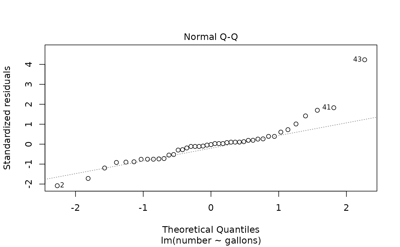
plot(model, which = 2)