SAT scores, percent taking exam and state funding per student by state for 1994, 1995 and 1999

Data for Statistical Insight Chapter 9

Sat

Format

A data frame/tibble with 102 observations on seven variables

state: U.S. state
verbal: verbal SAT score
math: math SAT score
total: combined verbal and math SAT score
percent: percent of high school seniors taking the SAT
expend: state expenditure per student (in dollars)
year: year

Source

The 2000 World Almanac and Book of Facts, Funk and Wagnalls Corporation, New Jersey.

References

Kitchens, L. J. (2003) Basic Statistics and Data Analysis. Pacific Grove, CA: Brooks/Cole, a division of Thomson Learning.

Examples


Sat94 <- Sat[Sat$year == 1994, ]
Sat94
#> # A tibble: 51 × 7
#>    state            verbal  math total percent expend year 
#>    <chr>             <int> <int> <int>   <int>  <int> <fct>
#>  1 alabama             482   529  1011       8   3616 1994 
#>  2 alaska              434   477   911      49   8450 1994 
#>  3 arizona             443   496   939      26   4381 1994 
#>  4 arkansas            417   518   935       6   4031 1994 
#>  5 california          413   482   895      46   4746 1994 
#>  6 colorado            456   513   969      28   5172 1994 
#>  7 connecticut         426   472   898      80   8017 1994 
#>  8 delaware            428   464   892      68   6093 1994 
#>  9 dist of columbia    406   443   849      53   9549 1994 
#> 10 florida             413   466   879      49   5243 1994 
#> # ℹ 41 more rows
Sat99 <- subset(Sat, year == 1999)
Sat99
#> # A tibble: 51 × 7
#>    state            verbal  math total percent expend year 
#>    <chr>             <int> <int> <int>   <int>  <int> <fct>
#>  1 alabama             561   555  1116       9   4903 1999 
#>  2 alaska              516   514  1030      50   9097 1999 
#>  3 arizona             524   525  1049      34   4940 1999 
#>  4 arkansas            563   556  1119       6   4840 1999 
#>  5 california          497   514  1011      49   5414 1999 
#>  6 colorado            536   540  1076      32   5728 1999 
#>  7 connecticut         510   509  1019      80   8901 1999 
#>  8 delaware            503   497  1000      67   7804 1999 
#>  9 dist of columbia    494   478   972      77   9019 1999 
#> 10 florida             499   498   997      53   5986 1999 
#> # ℹ 41 more rows
stem(Sat99$total)
#> 
#>   The decimal point is 1 digit(s) to the right of the |
#> 
#>    94 | 4
#>    96 | 92
#>    98 | 6334577
#>   100 | 03780149
#>   102 | 029089
#>   104 | 901
#>   106 | 6
#>   108 | 21147
#>   110 | 212699
#>   112 | 2789
#>   114 | 444
#>   116 | 39
#>   118 | 429
#> 
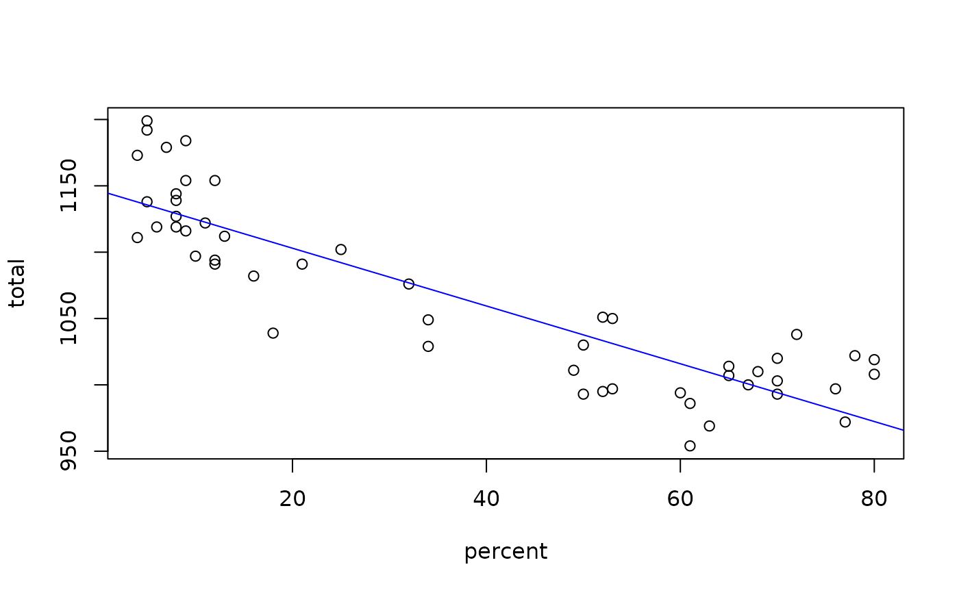
plot(total ~ percent, data = Sat99)
model <- lm(total ~ percent, data = Sat99)
abline(model, col = "blue")

summary(model)
#> 
#> Call:
#> lm(formula = total ~ percent, data = Sat99)
#> 
#> Residuals:
#>     Min      1Q  Median      3Q     Max 
#> -68.343 -26.613  -0.865  18.263  63.356 
#> 
#> Coefficients:
#>              Estimate Std. Error t value Pr(>|t|)    
#> (Intercept) 1146.5289     7.4940  152.99   <2e-16 ***
#> percent       -2.1770     0.1629  -13.37   <2e-16 ***
#> ---
#> Signif. codes:  0 ‘***’ 0.001 ‘**’ 0.01 ‘*’ 0.05 ‘.’ 0.1 ‘ ’ 1
#> 
#> Residual standard error: 31.81 on 49 degrees of freedom
#> Multiple R-squared:  0.7848,	Adjusted R-squared:  0.7804 
#> F-statistic: 178.7 on 1 and 49 DF,  p-value: < 2.2e-16
#> 
rm(model)