Oceanography data obtained at site 2 by scientist aboard the ship Ron Brown
Source:R/BSDA-package.R
Ronbrown2.RdData for Exercise 2.56 and Example 2.4
Ronbrown2Format
A data frame/tibble with 150 observations on three variables
- depth
ocean depth (in meters)
- temperature
ocean temperature (in Celcius)
- salinity
ocean salinity level
References
Kitchens, L. J. (2003) Basic Statistics and Data Analysis. Pacific Grove, CA: Brooks/Cole, a division of Thomson Learning.
Examples
plot(salinity ~ depth, data = Ronbrown2)
 model <- lm(salinity ~ depth, data = Ronbrown2)
summary(model)
#>
#> Call:
#> lm(formula = salinity ~ depth, data = Ronbrown2)
#>
#> Residuals:
#> Min 1Q Median 3Q Max
#> -0.15739 -0.12286 -0.09847 0.09494 0.44750
#>
#> Coefficients:
#> Estimate Std. Error t value Pr(>|t|)
#> (Intercept) 3.520e+01 2.702e-02 1302.97 <2e-16 ***
#> depth -9.212e-04 5.332e-05 -17.28 <2e-16 ***
#> ---
#> Signif. codes: 0 ‘***’ 0.001 ‘**’ 0.01 ‘*’ 0.05 ‘.’ 0.1 ‘ ’ 1
#>
#> Residual standard error: 0.1818 on 148 degrees of freedom
#> Multiple R-squared: 0.6685, Adjusted R-squared: 0.6663
#> F-statistic: 298.5 on 1 and 148 DF, p-value: < 2.2e-16
#>
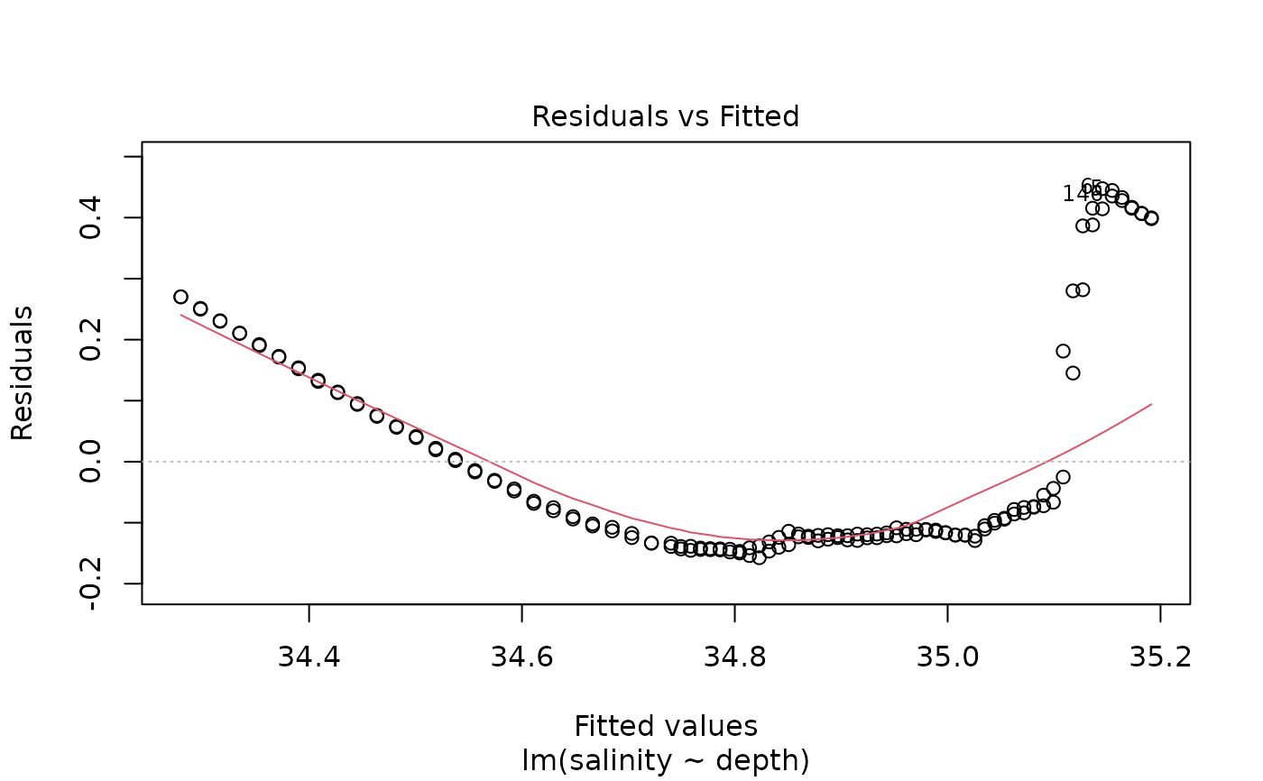
plot(model, which = 1)
model <- lm(salinity ~ depth, data = Ronbrown2)
summary(model)
#>
#> Call:
#> lm(formula = salinity ~ depth, data = Ronbrown2)
#>
#> Residuals:
#> Min 1Q Median 3Q Max
#> -0.15739 -0.12286 -0.09847 0.09494 0.44750
#>
#> Coefficients:
#> Estimate Std. Error t value Pr(>|t|)
#> (Intercept) 3.520e+01 2.702e-02 1302.97 <2e-16 ***
#> depth -9.212e-04 5.332e-05 -17.28 <2e-16 ***
#> ---
#> Signif. codes: 0 ‘***’ 0.001 ‘**’ 0.01 ‘*’ 0.05 ‘.’ 0.1 ‘ ’ 1
#>
#> Residual standard error: 0.1818 on 148 degrees of freedom
#> Multiple R-squared: 0.6685, Adjusted R-squared: 0.6663
#> F-statistic: 298.5 on 1 and 148 DF, p-value: < 2.2e-16
#>
plot(model, which = 1)
 rm(model)