Percent of marked cars in 65 police departments in Florida

Data for Exercise 6.100

Marked

Format

A data frame/tibble with 65 observations on one variable

percent

percentage of marked cars in 65 Florida police departments

Source

Law Enforcement Management and Administrative Statistics, 1993, Bureau of Justice Statistics, NCJ-148825, September 1995, p. 147-148.

References

Kitchens, L. J. (2003) Basic Statistics and Data Analysis. Pacific Grove, CA: Brooks/Cole, a division of Thomson Learning.

Examples

EDA(Marked$percent)
#> [1] "Marked$percent"

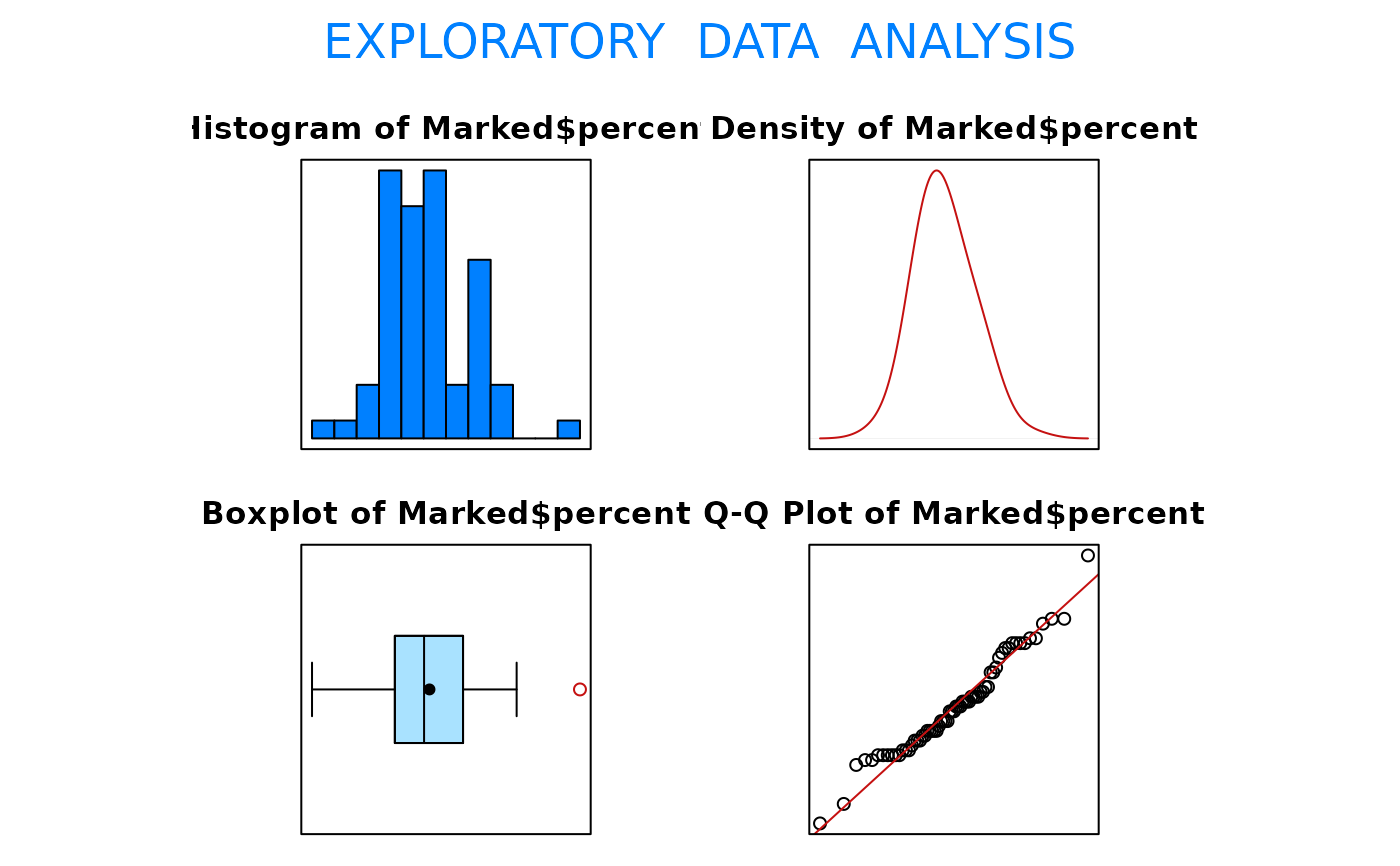#> Size (n)  Missing  Minimum   1st Qu     Mean   Median   TrMean   3rd Qu 
#>   65.000    0.000   37.000   54.000   61.108   60.000   60.932   68.000 
#>     Max.   Stdev.     Var.  SE Mean   I.Q.R.    Range Kurtosis Skewness 
#>   92.000    9.980   99.598    1.238   14.000   55.000    0.273    0.443 
#> SW p-val 
#>    0.072 
SIGN.test(Marked$percent, md = 60, alternative = "greater")
#> 
#> 	One-sample Sign-Test
#> 
#> data:  Marked$percent
#> s = 32, p-value = 0.4495
#> alternative hypothesis: true median is greater than 60
#> 95 percent confidence interval:
#>  57.33704      Inf
#> sample estimates:
#> median of x 
#>          60 
#> 
#> Achieved and Interpolated Confidence Intervals: 
#> 
#>                   Conf.Level L.E.pt U.E.pt
#> Lower Achieved CI     0.9320 58.000    Inf
#> Interpolated CI       0.9500 57.337    Inf
#> Upper Achieved CI     0.9592 57.000    Inf
#> 
t.test(Marked$percent, mu = 60, alternative = "greater")
#> 
#> 	One Sample t-test
#> 
#> data:  Marked$percent
#> t = 0.89485, df = 64, p-value = 0.1871
#> alternative hypothesis: true mean is greater than 60
#> 95 percent confidence interval:
#>  59.04171      Inf
#> sample estimates:
#> mean of x 
#>  61.10769 
#>