Data for Exercise 2.14, 2.17, 2.31, 2.33, and 2.40
JdpowerFormat
A data frame/tibble with 29 observations on three variables
- car
a factor with levels
Acura,BMW,Buick,Cadillac,Chevrolet,DodgeEagle,Ford,Geo,Honda,Hyundai,Infiniti,Jaguar,Lexus,Lincoln,Mazda,Mercedes-Benz,Mercury,Mitsubishi,Nissan,Oldsmobile,Plymouth,Pontiac,Saab,Saturn, andSubaru,ToyotaVolkswagen,Volvo- 1994
number of problems per 100 cars in 1994
- 1995
number of problems per 100 cars in 1995
Source
USA Today, May 25, 1995.
References
Kitchens, L. J. (2003) Basic Statistics and Data Analysis. Pacific Grove, CA: Brooks/Cole, a division of Thomson Learning.
Examples
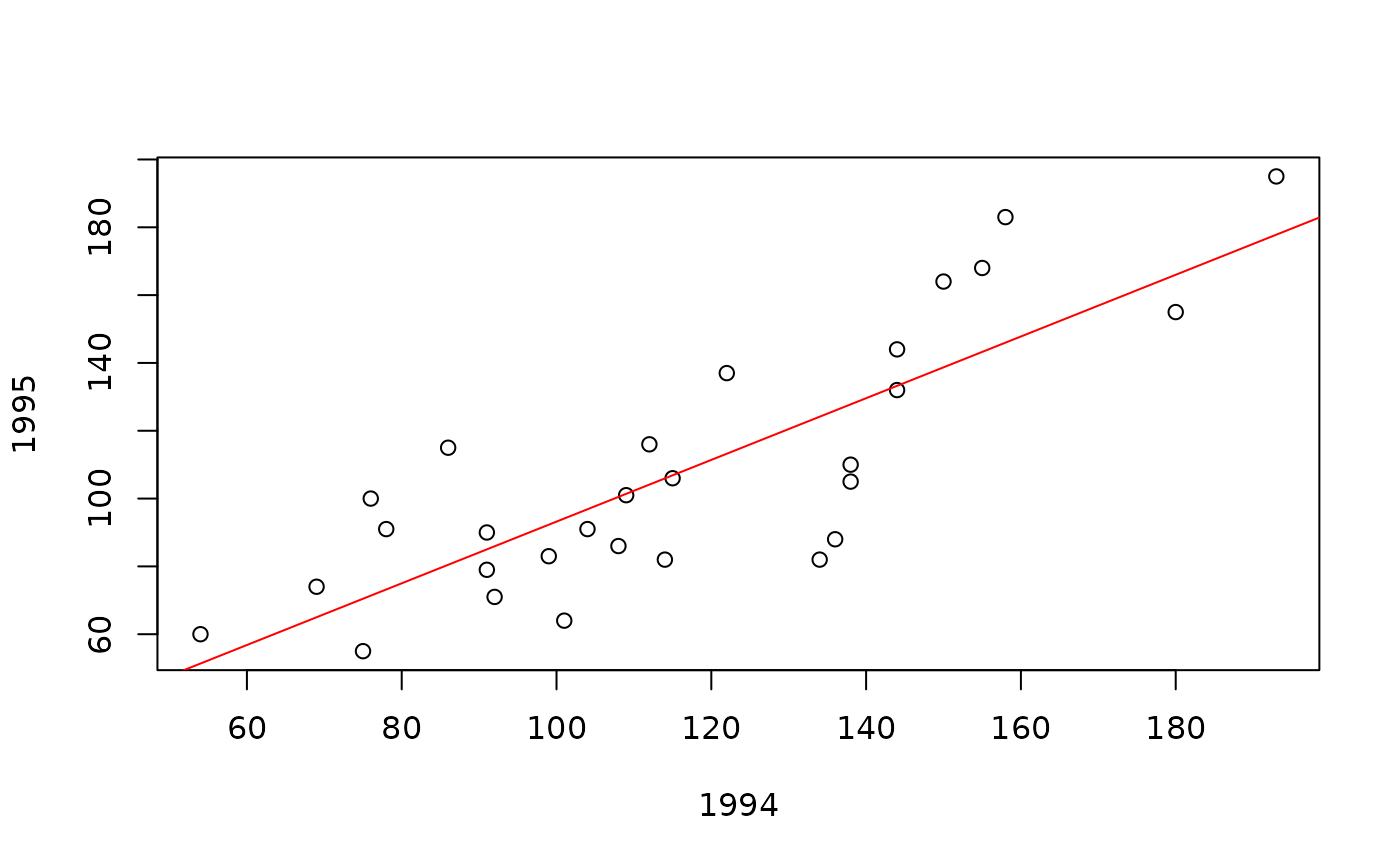
model <- lm(`1995` ~ `1994`, data = Jdpower)
summary(model)
#>
#> Call:
#> lm(formula = `1995` ~ `1994`, data = Jdpower)
#>
#> Residuals:
#>     Min      1Q  Median      3Q     Max
#> -42.142 -14.929  -0.855  17.178  37.022
#>
#> Coefficients:
#>             Estimate Std. Error t value Pr(>|t|)
#> (Intercept)   2.2241    14.6449   0.152     0.88
#> `1994`        0.9098     0.1213   7.501 4.55e-08 ***
#> ---
#> Signif. codes:  0 ‘***’ 0.001 ‘**’ 0.01 ‘*’ 0.05 ‘.’ 0.1 ‘ ’ 1
#>
#> Residual standard error: 21.72 on 27 degrees of freedom
#> Multiple R-squared:  0.6757,	Adjusted R-squared:  0.6637
#> F-statistic: 56.26 on 1 and 27 DF,  p-value: 4.546e-08
#>
plot(`1995` ~ `1994`, data = Jdpower)
abline(model, col = "red")

rm(model)