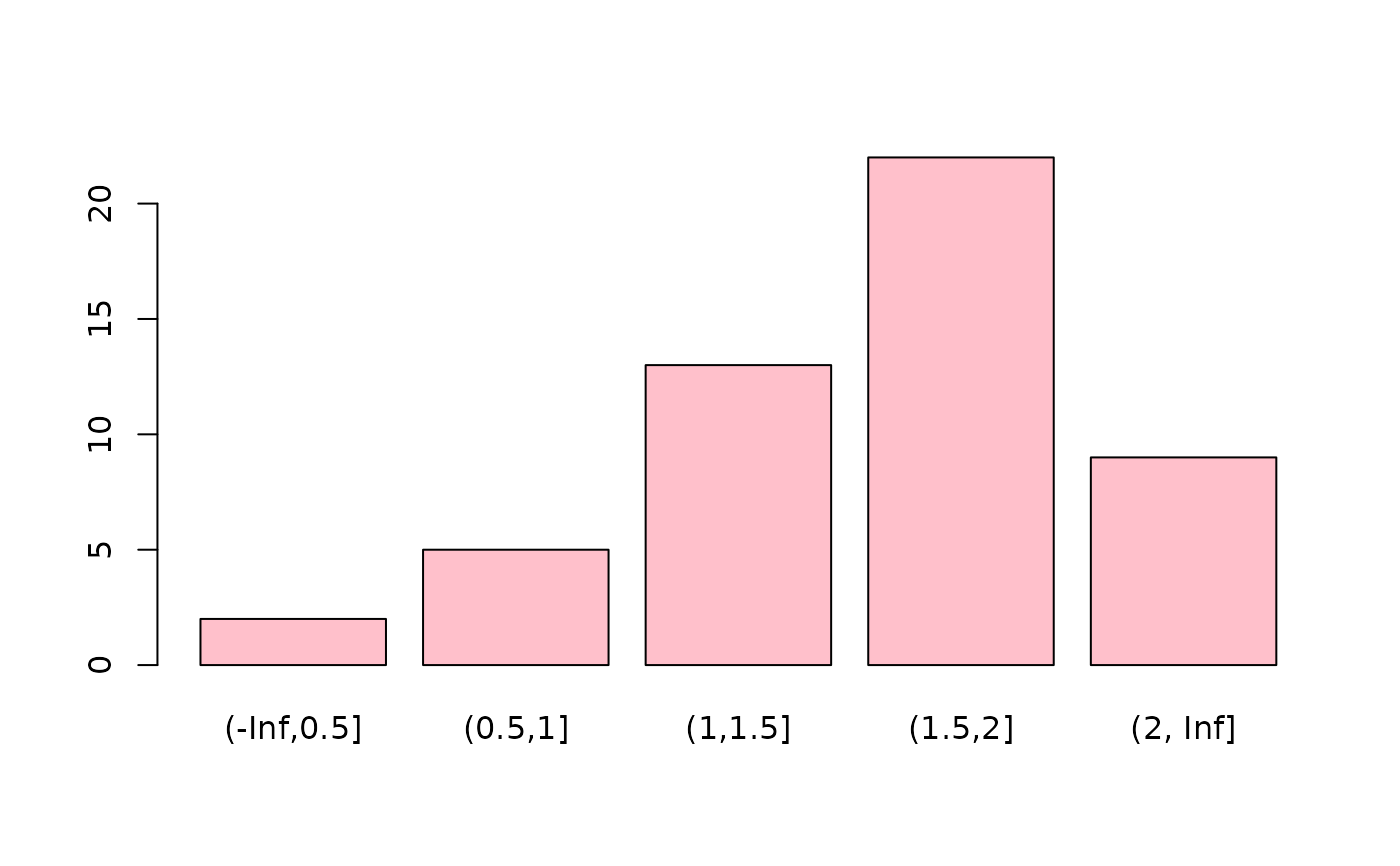
Percent change in personal income from 1st to 2nd quarter in 2000

Data for Exercise 1.33

Income

Format

A data frame/tibble with 51 observations on two variables

state

a character variable with values Alabama, Alaska, Arizona, Arkansas, California, Colorado, Connecticut, Delaware, District of Colunbia, Florida, Georgia, Hawaii, Idaho, Illinois, Indiana, Iowa, Kansas, Kentucky, Louisiana, Maine, Maryland, Massachusetts, Michigan, Minnesota, Mississippi, Missour, Montana, Nebraska, Nevada, New Hampshire, New Jersey, New Mexico, New York, North Carolina, North Dakota, Ohio, Oklahoma, Oregon, Pennsylvania, Rhode Island, South Carolina, South Dakota, Tennessee, Texas, Utah, Vermont, Virginia, Washington, West Virginia, Wisconsin, and Wyoming

percent_change

percent change in income from first quarter to the second quarter of 2000

Source

US Department of Commerce.

References

Kitchens, L. J. (2003) Basic Statistics and Data Analysis. Pacific Grove, CA: Brooks/Cole, a division of Thomson Learning.

Examples

Income$class <- cut(Income$percent_change, 
                    breaks = c(-Inf, 0.5, 1.0, 1.5, 2.0, Inf))
T1 <- xtabs(~class, data = Income)
T1
#> class
#> (-Inf,0.5]    (0.5,1]    (1,1.5]    (1.5,2]   (2, Inf] 
#>          2          5         13         22          9 
barplot(T1, col = "pink")   

if (FALSE) {
library(ggplot2)
DF <- as.data.frame(T1)
DF
ggplot2::ggplot(data = DF,  aes(x = class, y = Freq)) + 
           geom_bar(stat = "identity", fill = "purple") + 
           theme_bw()
}