Measurements of the thickness of the oxide layer of manufactured integrated circuits
Source:R/BSDA-package.R
Chipavg.RdData for Exercises 6.49 and 7.47
ChipavgFormat
A data frame/tibble with 30 observations on three variables
- wafer1
thickness of the oxide layer for
wafer1- wafer2
thickness of the oxide layer for
wafer2- thickness
average thickness of the oxide layer of the eight measurements obtained from each set of two wafers
Source
Yashchin, E. 1995. “Likelihood Ratio Methods for Monitoring Parameters of a Nested Random Effect Model.” Journal of the American Statistical Association, 90, 729-738.
References
Kitchens, L. J. (2003) Basic Statistics and Data Analysis. Pacific Grove, CA: Brooks/Cole, a division of Thomson Learning.
Examples
EDA(Chipavg$thickness)
#> [1] "Chipavg$thickness"
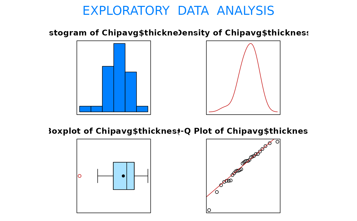 #> Size (n) Missing Minimum 1st Qu Mean Median TrMean 3rd Qu
#> 30.000 0.000 865.000 981.562 1016.333 1028.125 1018.705 1054.062
#> Max. Stdev. Var. SE Mean I.Q.R. Range Kurtosis Skewness
#> 1101.250 52.954 2804.088 9.668 72.500 236.250 0.308 -0.653
#> SW p-val
#> 0.339
t.test(Chipavg$thickness, mu = 1000)
#>
#> One Sample t-test
#>
#> data: Chipavg$thickness
#> t = 1.6894, df = 29, p-value = 0.1019
#> alternative hypothesis: true mean is not equal to 1000
#> 95 percent confidence interval:
#> 996.5601 1036.1065
#> sample estimates:
#> mean of x
#> 1016.333
#>
boxplot(Chipavg$wafer1, Chipavg$wafer2, name = c("Wafer 1", "Wafer 2"))
#> Size (n) Missing Minimum 1st Qu Mean Median TrMean 3rd Qu
#> 30.000 0.000 865.000 981.562 1016.333 1028.125 1018.705 1054.062
#> Max. Stdev. Var. SE Mean I.Q.R. Range Kurtosis Skewness
#> 1101.250 52.954 2804.088 9.668 72.500 236.250 0.308 -0.653
#> SW p-val
#> 0.339
t.test(Chipavg$thickness, mu = 1000)
#>
#> One Sample t-test
#>
#> data: Chipavg$thickness
#> t = 1.6894, df = 29, p-value = 0.1019
#> alternative hypothesis: true mean is not equal to 1000
#> 95 percent confidence interval:
#> 996.5601 1036.1065
#> sample estimates:
#> mean of x
#> 1016.333
#>
boxplot(Chipavg$wafer1, Chipavg$wafer2, name = c("Wafer 1", "Wafer 2"))
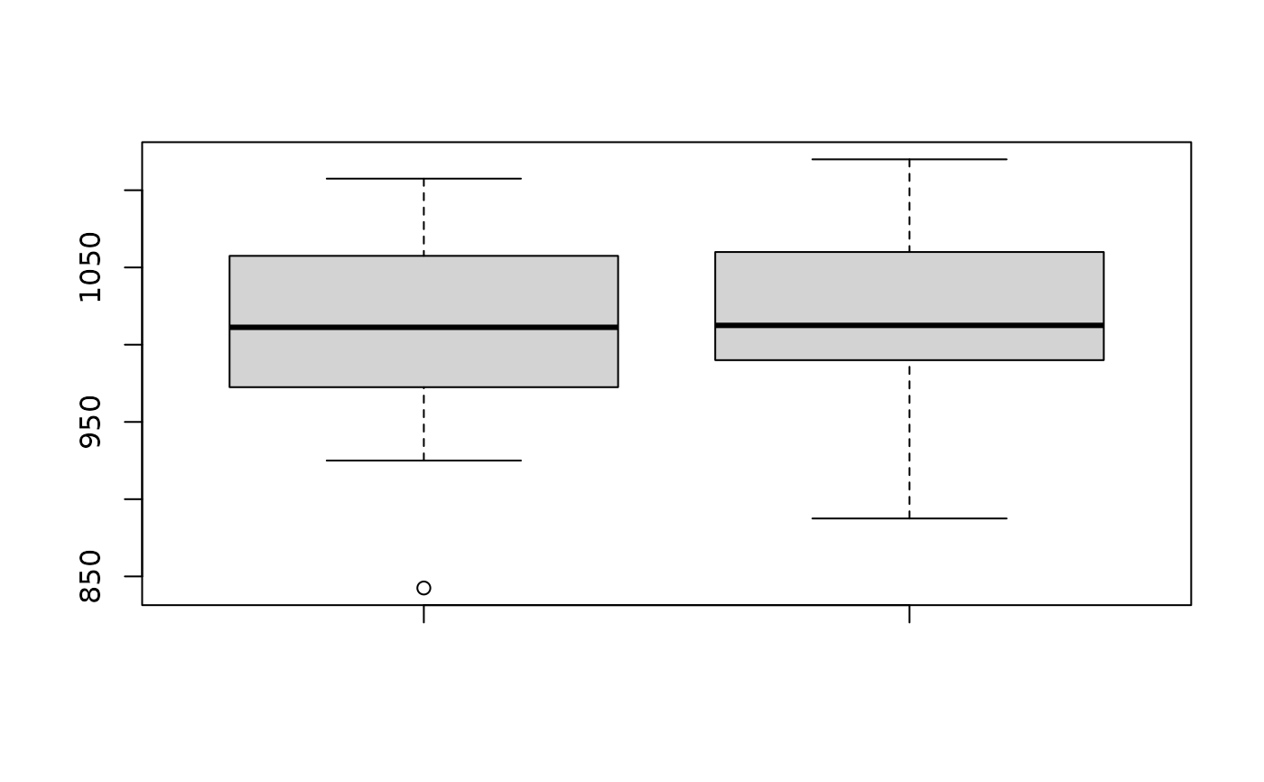 shapiro.test(Chipavg$wafer1)
#>
#> Shapiro-Wilk normality test
#>
#> data: Chipavg$wafer1
#> W = 0.9545, p-value = 0.2228
#>
shapiro.test(Chipavg$wafer2)
#>
#> Shapiro-Wilk normality test
#>
#> data: Chipavg$wafer2
#> W = 0.96426, p-value = 0.3959
#>
t.test(Chipavg$wafer1, Chipavg$wafer2, var.equal = TRUE)
#>
#> Two Sample t-test
#>
#> data: Chipavg$wafer1 and Chipavg$wafer2
#> t = -0.55603, df = 58, p-value = 0.5803
#> alternative hypothesis: true difference in means is not equal to 0
#> 95 percent confidence interval:
#> -39.10005 22.10005
#> sample estimates:
#> mean of x mean of y
#> 1012.083 1020.583
#>
shapiro.test(Chipavg$wafer1)
#>
#> Shapiro-Wilk normality test
#>
#> data: Chipavg$wafer1
#> W = 0.9545, p-value = 0.2228
#>
shapiro.test(Chipavg$wafer2)
#>
#> Shapiro-Wilk normality test
#>
#> data: Chipavg$wafer2
#> W = 0.96426, p-value = 0.3959
#>
t.test(Chipavg$wafer1, Chipavg$wafer2, var.equal = TRUE)
#>
#> Two Sample t-test
#>
#> data: Chipavg$wafer1 and Chipavg$wafer2
#> t = -0.55603, df = 58, p-value = 0.5803
#> alternative hypothesis: true difference in means is not equal to 0
#> 95 percent confidence interval:
#> -39.10005 22.10005
#> sample estimates:
#> mean of x mean of y
#> 1012.083 1020.583
#>