Data for Example 1.10
BirthFormat
A data frame/tibble with 51 observations on three variables
- state
a character with levels
Alabama,Alaska,Arizona,Arkansas,California,Colorado,Connecticut,Delaware,District of Colunbia,Florida,Georgia,Hawaii,Idaho,Illinois,Indiana,Iowa,Kansas,Kentucky,Louisiana,Maine,Maryland,Massachusetts,Michigan,Minnesota,Mississippi,Missour,Montana,Nebraska,Nevada,New Hampshire,New Jersey,New Mexico,New York,North Carolina,North Dakota,Ohio,Oklahoma,Oregon,Pennsylvania,Rhode Island,South Carolina,South Dakota,Tennessee,Texas,Utah,Vermont,Virginia,Washington,West Virginia,Wisconsin, andWyoming- rate
live birth rates per 1000 population
- year
a factor with levels
1990and1998
Source
National Vital Statistics Report, 48, March 28, 2000, National Center for Health Statistics.
References
Kitchens, L. J. (2003) Basic Statistics and Data Analysis. Pacific Grove, CA: Brooks/Cole, a division of Thomson Learning.
Examples
rate1998 <- subset(Birth, year == "1998", select = rate)
stem(x = rate1998$rate, scale = 2)
#>
#> The decimal point is at the |
#>
#> 11 | 015
#> 12 | 223479
#> 13 | 0012466888999
#> 14 | 0001222334567788
#> 15 | 023678
#> 16 | 00248
#> 17 | 3
#> 18 |
#> 19 |
#> 20 |
#> 21 | 5
#>
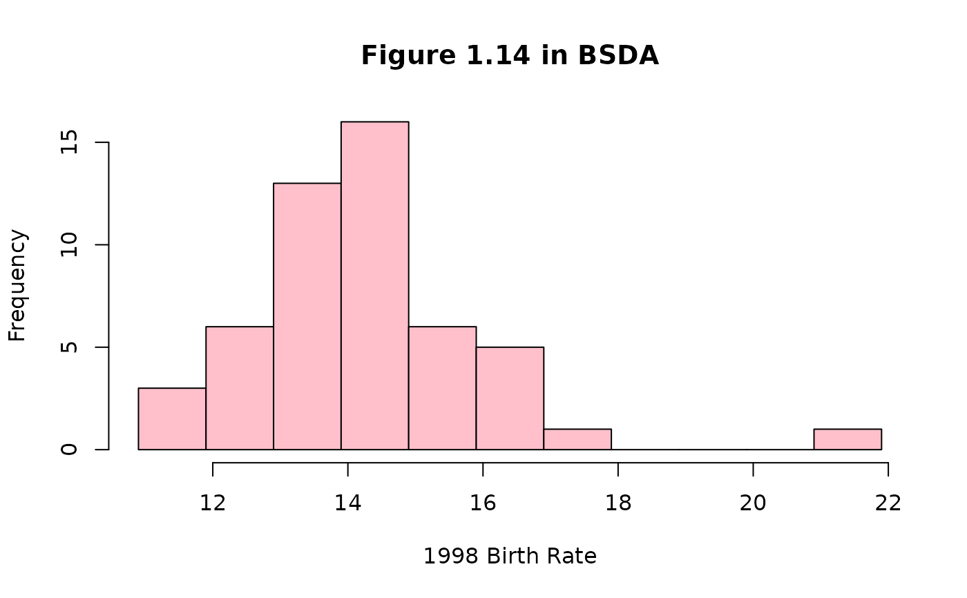
hist(rate1998$rate, breaks = seq(10.9, 21.9, 1.0), xlab = "1998 Birth Rate",
main = "Figure 1.14 in BSDA", col = "pink")
 hist(rate1998$rate, breaks = seq(10.9, 21.9, 1.0), xlab = "1998 Birth Rate",
main = "Figure 1.16 in BSDA", col = "pink", freq = FALSE)
lines(density(rate1998$rate), lwd = 3)
hist(rate1998$rate, breaks = seq(10.9, 21.9, 1.0), xlab = "1998 Birth Rate",
main = "Figure 1.16 in BSDA", col = "pink", freq = FALSE)
lines(density(rate1998$rate), lwd = 3)
 rm(rate1998)